library(SeroTrackR)
library(tidyverse)

your_raw_data <- c(
  system.file("extdata", "example_MAGPIX_plate1.csv", package = "SeroTrackR"),
  system.file("extdata", "example_MAGPIX_plate2.csv", package = "SeroTrackR"),
  system.file("extdata", "example_MAGPIX_plate3.csv", package = "SeroTrackR")
)
your_plate_layout <- system.file("extdata", "example_platelayout_1.xlsx", package = "SeroTrackR")1 PvSeroApp in R Tutorial
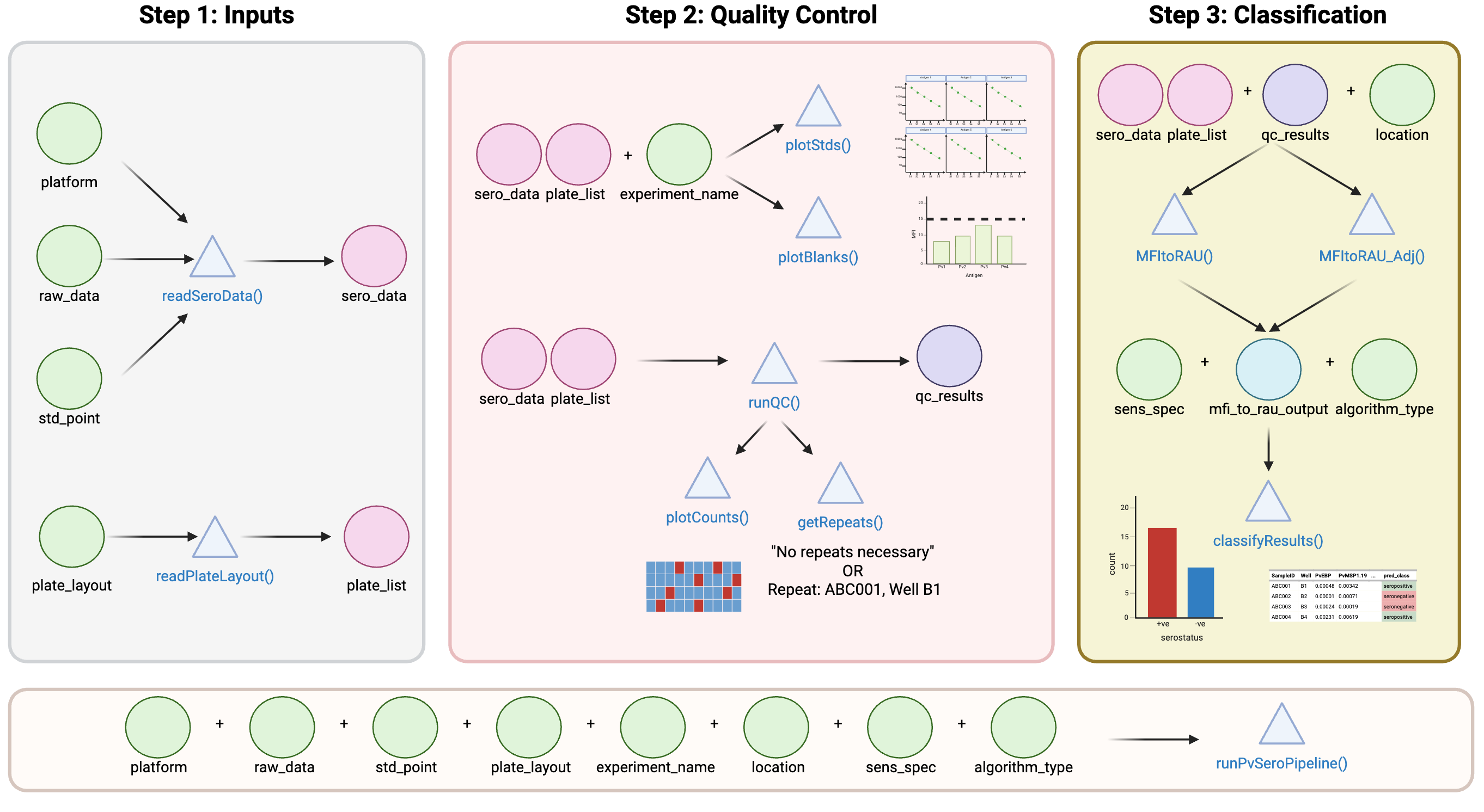
1.1 Data Analysis: function by function
We can also run the functions within the runPvSeroPipeline() to identify each step independently. This can be useful particularly when modifying graphs or saving files and interrogating the data.
1.1.1 Visualisation of the PvSeroApp Pipeline
1.1.2 Using Tutorial Dataset: Load the Data
We will be using the build-in files in the R package for this tutorial, as shown here:
To run your OWN data, follow the code here, replacing PATH/TO/YOUR/FILE with your file path:
your_raw_data <- c(
  "PATH/TO/YOUR/FILE/plate1.csv",
  "PATH/TO/YOUR/FILE/plate2.csv",
  "PATH/TO/YOUR/FILE/plate3.csv"
)
your_plate_layout <- "PATH/TO/YOUR/FILE/plate_layout.xlsx"
NoteData preparation
Please ensure that you have read and prepared your raw Luminex files and plate layout files as per the instructions in the Before You Begin page.
1.1.3 Step 1: Read in the raw data
You can read any Luminex serology data file using the readSeroData() function.
The Luminex platform can be specified using the platform argument, with either bioplex, magpix or intelliflex.
For the xPONENT software-based exported files (MAGPIX or INTELLIFLEX), the version of the software should be specified as either “4.2” or “4.3”, with the version “4.2” as the default.
sero_data <- readSeroData(
  raw_data = your_raw_data,
  platform = "magpix",        # default
  version = "4.2"             # default
)
#> PASS: File example_magpix_plate1.csv successfully validated.
#> PASS: File example_magpix_plate2.csv successfully validated.
#> PASS: File example_magpix_plate3.csv successfully validated.sero_data$ data_raw
| Program | xPONENT | X | MAGPIX | X.1 | X.2 | X.3 | X.4 | X.5 | X.6 | X.7 | X.8 | X.9 | X.10 | X.11 | X.12 | X.13 | Plate |
|---|---|---|---|---|---|---|---|---|---|---|---|---|---|---|---|---|---|
| Build | 4.2.1705.0 | plate1 | |||||||||||||||
| Date | 1/1/2024 | 11:11 am | plate1 | ||||||||||||||
| plate1 | |||||||||||||||||
| SN | MAGPX17087723 | plate1 | |||||||||||||||
| Batch | Example_Plate | plate1 | |||||||||||||||
| Version | 1 | plate1 | |||||||||||||||
| Operator | DA | plate1 | |||||||||||||||
| ComputerName | MAGPIX-PC | plate1 | |||||||||||||||
| Country Code | 409 | plate1 | |||||||||||||||
| ProtocolName | PvSeroTaT_v1.0 | plate1 | |||||||||||||||
| ProtocolVersion | 1 | plate1 | |||||||||||||||
| ProtocolDescription | plate1 | ||||||||||||||||
| ProtocolDevelopingCompany | plate1 | ||||||||||||||||
| SampleWash | Off | plate1 | |||||||||||||||
| SampleVolume | 75 uL | plate1 | |||||||||||||||
| BatchStartTime | 1/1/2024 11:11 | plate1 | |||||||||||||||
| BatchStopTime | 1/1/2024 12:11 | plate1 | |||||||||||||||
| BatchDescription | <None> | plate1 | |||||||||||||||
| ProtocolPlate | Name | Current 96-well plate | Type | 96 | Plates | 1 | plate1 | ||||||||||
| ProtocolMicrosphere | Map | BP 50 regions | Type | MagPlex | Count | 18 | plate1 | ||||||||||
| ProtocolAnalysis | Off | plate1 | |||||||||||||||
| NormBead | None | plate1 | |||||||||||||||
| ProtocolHeater | Off | plate1 | |||||||||||||||
| plate1 | |||||||||||||||||
| Most Recent Calibration and Verification Results: | plate1 | ||||||||||||||||
| Last CAL Calibration | Passed 01/01/2024 12:11:11 | plate1 | |||||||||||||||
| Last VER Verification | Passed 01/01/2024 12:11:11 | plate1 | |||||||||||||||
| Last Fluidics Test | Passed 01/01/2024 12:11:11 | plate1 | |||||||||||||||
| plate1 | |||||||||||||||||
| CALInfo: | plate1 | ||||||||||||||||
| Calibrator | plate1 | ||||||||||||||||
| Lot | ExpirationDate | CalibrationTime | CL1Temp | CL2Temp | RP1LongTemp | RP1ShortTemp | CL1Current | CL2Current | RP1LongCurrent | RP1ShortCurrent | CL1Factor | CL2Factor | RP1LongFactor | RP1ShortFactor | Result | MachineSerialNo | plate1 |
| C00921 | 03/20/2025 | 11/20/2024 2:43:32 PM | 35.6 | 35.6 | 35.6 | 35.6 | 240 | 248 | 313 | 313 | 0.00707 | 0.00707 | 0.00395 | 0.11659 | Pass | MAGPX17087723 | plate1 |
| plate1 | |||||||||||||||||
| plate1 | |||||||||||||||||
| Samples | 96 | Min Events | 50 | Per Bead | plate1 | ||||||||||||
| plate1 | |||||||||||||||||
| Results | plate1 | ||||||||||||||||
| plate1 | |||||||||||||||||
| DataType: | Median | plate1 | |||||||||||||||
| Location | Sample | EBP | LF005 | LF010 | LF016 | MSP8 | RBP2b.P87 | PTEX150 | PvCSS | Total Events | plate1 | ||||||
| 1(1,A1) | Blank1 | 20 | 200 | 20 | 10 | 20 | 10 | 30 | 20 | 1898 | plate1 | ||||||
| 2(1,A2) | Blank2 | 15 | 291 | 15 | 15 | 15 | 10 | 20 | 15 | 1805 | plate1 | ||||||
| 3(1,A3) | S1 | 15710.5 | 11990 | 22583 | 21244 | 24306 | 7907.5 | 13207 | 12427 | 1842 | plate1 | ||||||
| 4(1,A4) | S2 | 13545 | 8285 | 16947.5 | 16146 | 17172 | 7186 | 8550 | 8034 | 2044 | plate1 | ||||||
| 5(1,A5) | S3 | 9767 | 4950 | 10865 | 10621.5 | 11358 | 4475.5 | 5329 | 4990 | 1815 | plate1 | ||||||
| 6(1,A6) | S4 | 5648.5 | 2519 | 6060 | 5968.5 | 6237 | 3508 | 2671 | 2446.5 | 1950 | plate1 | ||||||
| 7(1,A7) | S5 | 4104.5 | 1431 | 3711.5 | 3738 | 3883.5 | 2082 | 1548 | 1299 | 1991 | plate1 | ||||||
| 8(1,A8) | S6 | 2105 | 676.5 | 1889 | 1667 | 2136 | 1102 | 698.5 | 581 | 1827 | plate1 | ||||||
| 9(1,A9) | S7 | 1107 | 328 | 1106 | 890 | 1204 | 657 | 333 | 264 | 2095 | plate1 | ||||||
| 10(1,A10) | S8 | 452.5 | 141 | 465 | 405.5 | 522 | 277 | 156 | 111 | 1643 | plate1 | ||||||
| 11(1,A11) | S9 | 209 | 65 | 206.5 | 181.5 | 249 | 138 | 77 | 46.5 | 1888 | plate1 | ||||||
| 12(1,A12) | S10 | 105 | 42 | 113.5 | 87 | 134 | 93 | 40 | 28 | 1876 | plate1 | ||||||
| 13(1,B1) | Unknown013 | 2712 | 1569 | 673 | 327 | 182 | 1068 | 936 | 223 | 1927 | plate1 | ||||||
| 14(1,B2) | Unknown014 | 134 | 378 | 117 | 197 | 58 | 465.5 | 122 | 93 | 1965 | plate1 | ||||||
| 15(1,B3) | Unknown015 | 182 | 209 | 208 | 374 | 221.5 | 463 | 293 | 868 | 1970 | plate1 | ||||||
| 16(1,B4) | Unknown016 | 152 | 229.5 | 101 | 89 | 48 | 591 | 109 | 110 | 1911 | plate1 | ||||||
| 17(1,B5) | Unknown017 | 1135 | 236 | 299 | 507 | 209.5 | 671 | 1665.5 | 266 | 1977 | plate1 | ||||||
| 18(1,B6) | Unknown018 | 174 | 395 | 175 | 78 | 70 | 103 | 294.5 | 92 | 1902 | plate1 | ||||||
| 19(1,B7) | Unknown019 | 421 | 2081.5 | 529 | 149 | 962 | 1441.5 | 241 | 282 | 1913 | plate1 | ||||||
| 20(1,B8) | Unknown020 | 24 | 49 | 22 | 13 | 15.5 | 14 | 28 | 17 | 1828 | plate1 | ||||||
| 21(1,B9) | Unknown021 | 24 | 45 | 22 | 13 | 16 | 13 | 29 | 17 | 1885 | plate1 | ||||||
| 22(1,B10) | Unknown022 | 21464 | 11789 | 2508.5 | 8001 | 2342 | 1386 | 1992 | 2927 | 2133 | plate1 | ||||||
| 23(1,B11) | Unknown023 | 795 | 6135.5 | 407 | 273 | 535.5 | 1575 | 8821 | 998 | 1670 | plate1 | ||||||
| 24(1,B12) | Unknown024 | 1574 | 348.5 | 892 | 288 | 306 | 590 | 315 | 366 | 1955 | plate1 | ||||||
| 25(1,C1) | Unknown025 | 146 | 408.5 | 1130.5 | 83 | 100 | 301 | 652 | 130 | 1873 | plate1 | ||||||
| 26(1,C2) | Unknown026 | 1330.5 | 3036 | 965 | 174 | 79 | 1090 | 179 | 92 | 2173 | plate1 | ||||||
| 27(1,C3) | Unknown027 | 358 | 4074.5 | 335.5 | 140 | 390 | 6704 | 8814 | 5627 | 2012 | plate1 | ||||||
| 28(1,C4) | Unknown028 | 481 | 1870 | 421 | 182.5 | 1777.5 | 2390 | 2465 | 411 | 1794 | plate1 | ||||||
| 29(1,C5) | Unknown029 | 551 | 1282 | 331.5 | 165 | 77 | 244 | 579 | 229 | 2023 | plate1 | ||||||
| 30(1,C6) | Unknown030 | 943 | 584.5 | 235 | 135 | 3017 | 1034 | 4928 | 7730 | 1893 | plate1 | ||||||
| 31(1,C7) | Unknown031 | 532.5 | 1533 | 315 | 210 | 2575.5 | 2903 | 2779 | 7300 | 1946 | plate1 | ||||||
| 32(1,C8) | Unknown032 | 768 | 12605 | 409 | 7632 | 9860 | 13703 | 5612 | 6383 | 1843 | plate1 | ||||||
| 33(1,C9) | Unknown033 | 130 | 239.5 | 72 | 64 | 37 | 156 | 204 | 49 | 1900 | plate1 | ||||||
| 34(1,C10) | Unknown034 | 40 | 60 | 37 | 25 | 26.5 | 23.5 | 40 | 27 | 1947 | plate1 | ||||||
| 35(1,C11) | Unknown035 | 167 | 605 | 253 | 329 | 3973 | 1426.5 | 803 | 1670 | 1826 | plate1 | ||||||
| 36(1,C12) | Unknown036 | 1879 | 4562 | 415 | 18287 | 11482.5 | 12031 | 4830.5 | 4217 | 1690 | plate1 | ||||||
| 37(1,D1) | Unknown037 | 256 | 1507 | 117 | 129 | 168 | 488 | 908 | 87 | 1988 | plate1 | ||||||
| 38(1,D2) | Unknown038 | 24 | 49 | 22 | 12 | 15 | 14 | 29 | 17 | 1943 | plate1 | ||||||
| 39(1,D3) | Unknown039 | 384 | 1708 | 326 | 1172.5 | 986 | 1041 | 299.5 | 149 | 1963 | plate1 | ||||||
| 40(1,D4) | Unknown040 | 210 | 512 | 221 | 191 | 89 | 203 | 410 | 174.5 | 2159 | plate1 | ||||||
| 41(1,D5) | Unknown041 | 351.5 | 312 | 165.5 | 88 | 66 | 205 | 200 | 183 | 2122 | plate1 | ||||||
| 42(1,D6) | Unknown042 | 1278 | 5810 | 275 | 230.5 | 137 | 2032 | 1762 | 1241 | 1997 | plate1 | ||||||
| 43(1,D7) | Unknown043 | 318 | 397 | 130 | 130.5 | 78 | 903 | 1513.5 | 325 | 1916 | plate1 | ||||||
| 44(1,D8) | Unknown044 | 493.5 | 2980.5 | 401 | 5932.5 | 3536 | 4699.5 | 574 | 5389 | 2026 | plate1 | ||||||
| 45(1,D9) | Unknown045 | 9686 | 873 | 333 | 166 | 791 | 1093 | 417.5 | 262 | 1691 | plate1 | ||||||
| 46(1,D10) | Unknown046 | 777.5 | 581 | 241.5 | 173 | 1479.5 | 899 | 1504 | 260 | 2044 | plate1 | ||||||
| 47(1,D11) | Unknown047 | 455 | 416.5 | 126 | 67 | 48 | 400 | 183 | 61 | 1639 | plate1 | ||||||
| 48(1,D12) | Unknown048 | 202 | 1142 | 137.5 | 176 | 204.5 | 1090 | 504 | 459 | 1957 | plate1 | ||||||
| 49(1,E1) | Unknown049 | 333.5 | 623.5 | 368 | 10430 | 2340 | 4375 | 1650 | 7801.5 | 1836 | plate1 | ||||||
| 50(1,E2) | Unknown050 | 561 | 7984 | 441 | 128 | 141 | 1993 | 2147 | 1502 | 1963 | plate1 | ||||||
| 51(1,E3) | Unknown051 | 506.5 | 340 | 152.5 | 147 | 90 | 600 | 2178 | 170 | 1856 | plate1 | ||||||
| 52(1,E4) | Unknown052 | 254 | 367 | 392.5 | 89 | 142.5 | 280 | 298 | 138 | 2019 | plate1 | ||||||
| 53(1,E5) | Unknown053 | 888 | 1955 | 438 | 173 | 507 | 1009 | 709 | 2040 | 2009 | plate1 | ||||||
| 54(1,E6) | Unknown054 | 426 | 1877 | 186 | 9767 | 15945 | 10073 | 1585.5 | 1124 | 1964 | plate1 | ||||||
| 55(1,E7) | Unknown055 | 5733 | 1301.5 | 1920.5 | 220.5 | 4833 | 2340 | 5329 | 2369 | 1905 | plate1 | ||||||
| 56(1,E8) | Unknown056 | 19092 | 14422 | 1993 | 12836.5 | 7426 | 11930 | 4826 | 3468.5 | 2052 | plate1 | ||||||
| 57(1,E9) | Unknown057 | 596 | 15139 | 371.5 | 229 | 535.5 | 14032 | 7928.5 | 1414.5 | 1712 | plate1 | ||||||
| 58(1,E10) | Unknown058 | 1028 | 2646 | 1486 | 292 | 9357 | 8009 | 3736 | 14370.5 | 1862 | plate1 | ||||||
| 59(1,E11) | Unknown059 | 512 | 4735 | 3408 | 127.5 | 191 | 4401 | 11567 | 2923.5 | 1718 | plate1 | ||||||
| 60(1,E12) | Unknown060 | 883 | 1953 | 755 | 586 | 122 | 830 | 425.5 | 121 | 1767 | plate1 | ||||||
| 61(1,F1) | Unknown061 | 977 | 8719 | 509 | 187 | 1289 | 12930 | 13891 | 9531 | 1735 | plate1 | ||||||
| 62(1,F2) | Unknown062 | 791 | 1944 | 465 | 216.5 | 12307 | 5029 | 4157 | 760 | 1804 | plate1 | ||||||
| 63(1,F3) | Unknown063 | 397 | 987 | 924 | 133 | 79 | 253 | 2317.5 | 1080.5 | 1705 | plate1 | ||||||
| 64(1,F4) | Unknown064 | 1111 | 613 | 357 | 196 | 8496 | 7914 | 5772.5 | 13202 | 2026 | plate1 | ||||||
| 65(1,F5) | Unknown065 | 956 | 2369 | 644 | 389 | 8762 | 9649 | 6437 | 21113 | 1871 | plate1 | ||||||
| 66(1,F6) | Unknown066 | 1307 | 20590 | 1335 | 10780 | 12736 | 25375.5 | 5493 | 7696 | 1868 | plate1 | ||||||
| 67(1,F7) | Unknown067 | 433 | 382 | 173 | 105 | 59 | 480 | 655 | 367 | 1813 | plate1 | ||||||
| 68(1,F8) | Unknown068 | 161 | 279 | 2524.5 | 105.5 | 55 | 307 | 681.5 | 472.5 | 2070 | plate1 | ||||||
| 69(1,F9) | Unknown069 | 439 | 732.5 | 397 | 2108 | 9692 | 8090 | 9513 | 7341 | 1870 | plate1 | ||||||
| 70(1,F10) | Unknown070 | 1837 | 11406 | 467.5 | 20011 | 19606 | 24476.5 | 5822 | 5127.5 | 2055 | plate1 | ||||||
| 71(1,F11) | Unknown071 | 244 | 1665.5 | 166 | 124 | 154 | 224 | 718 | 115 | 1798 | plate1 | ||||||
| 72(1,F12) | Unknown072 | 482 | 3990.5 | 388 | 3736 | 7436 | 7361 | 4111.5 | 2819 | 1831 | plate1 | ||||||
| 73(1,G1) | Unknown073 | 656 | 3103 | 505 | 14386 | 2343 | 5503 | 357.5 | 1215 | 1816 | plate1 | ||||||
| 74(1,G2) | Unknown074 | 243 | 568.5 | 693 | 141 | 79 | 339 | 2080 | 1470 | 1821 | plate1 | ||||||
| 75(1,G3) | Unknown075 | 1409.5 | 1123 | 379 | 153 | 167.5 | 1013 | 1553 | 1738 | 1979 | plate1 | ||||||
| 76(1,G4) | Unknown076 | 467.5 | 6741 | 238 | 174 | 181 | 6160 | 1660.5 | 1087 | 1910 | plate1 | ||||||
| 77(1,G5) | Unknown077 | 329 | 630 | 196 | 119 | 278 | 787 | 2052.5 | 2221 | 1752 | plate1 | ||||||
| 78(1,G6) | Unknown078 | 1122.5 | 17810 | 677 | 12254 | 16011 | 18719 | 3551 | 10222.5 | 1670 | plate1 | ||||||
| 79(1,G7) | Unknown079 | 10853 | 817.5 | 255 | 189 | 2247.5 | 3322 | 590 | 258 | 1702 | plate1 | ||||||
| 80(1,G8) | Unknown080 | 743.5 | 820 | 313.5 | 289 | 9351.5 | 7171 | 3062 | 676.5 | 1739 | plate1 | ||||||
| 81(1,G9) | Unknown081 | 723 | 1255 | 299 | 253 | 95 | 712 | 396 | 129.5 | 1574 | plate1 | ||||||
| 82(1,G10) | Unknown082 | 168 | 684 | 131 | 198 | 135.5 | 392 | 292 | 254.5 | 1597 | plate1 | ||||||
| 83(1,G11) | Unknown083 | 180 | 276 | 205 | 4646.5 | 2550 | 2664.5 | 724 | 2707 | 1546 | plate1 | ||||||
| 84(1,G12) | Unknown084 | 249.5 | 4104 | 250 | 96 | 68 | 1020 | 960 | 672 | 1710 | plate1 | ||||||
| 85(1,H1) | Unknown085 | 479 | 190 | 105 | 131 | 66 | 1449 | 1724.5 | 108 | 2102 | plate1 | ||||||
| 86(1,H2) | Unknown086 | 164 | 327 | 234.5 | 66 | 75.5 | 259 | 260 | 89 | 1895 | plate1 | ||||||
| 87(1,H3) | Unknown087 | 281.5 | 1794 | 413 | 75 | 469.5 | 802 | 345 | 744.5 | 1694 | plate1 | ||||||
| 88(1,H4) | Unknown088 | 269 | 1067 | 141 | 7595 | 14464 | 7592 | 804.5 | 467 | 1817 | plate1 | ||||||
| 89(1,H5) | Unknown089 | 3247 | 382 | 470 | 98 | 2319.5 | 2009 | 1521 | 1258 | 1615 | plate1 | ||||||
| 90(1,H6) | Unknown090 | 20593 | 14902.5 | 2021 | 10184 | 5805.5 | 14083.5 | 4307.5 | 3073 | 1452 | plate1 | ||||||
| 91(1,H7) | Unknown091 | 395 | 9914 | 211 | 131.5 | 325 | 3021 | 4608 | 1073.5 | 1537 | plate1 | ||||||
| 92(1,H8) | Unknown092 | 904.5 | 1871 | 793 | 172 | 6106 | 2093 | 1303 | 6595.5 | 1852 | plate1 | ||||||
| 93(1,H9) | Unknown093 | 323 | 2007.5 | 1950 | 106 | 191 | 2411 | 7377.5 | 1699 | 1563 | plate1 | ||||||
| 94(1,H10) | Unknown094 | 706 | 2087 | 791 | 169 | 66 | 990 | 261 | 65 | 1472 | plate1 | ||||||
| 95(1,H11) | Unknown095 | 323 | 4950 | 264 | 107 | 645 | 7092 | 8856 | 5330 | 1467 | plate1 | ||||||
| 96(1,H12) | Unknown096 | 367 | 1067 | 259 | 101 | 7423 | 1203 | 1841.5 | 335 | 1654 | plate1 | ||||||
| plate1 | |||||||||||||||||
| DataType: | Net MFI | plate1 | |||||||||||||||
| Location | Sample | EBP | LF005 | LF010 | LF016 | MSP8 | RBP2b.P87 | PTEX150 | PvCSS | Total Events | plate1 | ||||||
| 1(1,A1) | Blank1 | 24 | 200 | 22 | 12 | 16 | 13 | 28 | 16 | 1898 | plate1 | ||||||
| 2(1,A2) | Blank2 | 20 | 291 | 24 | 15 | 17 | 11 | 24 | 15 | 1887 | plate1 | ||||||
| 3(1,A3) | S1 | 15710.5 | 11990 | 22583 | 21244 | 24306 | 7907.5 | 13207 | 12427 | 1842 | plate1 | ||||||
| 4(1,A4) | S2 | 13545 | 8285 | 16947.5 | 16146 | 17172 | 7186 | 8550 | 8034 | 2044 | plate1 | ||||||
| 5(1,A5) | S3 | 9767 | 4950 | 10865 | 10621.5 | 11358 | 4475.5 | 5329 | 4990 | 1815 | plate1 | ||||||
| 6(1,A6) | S4 | 5648.5 | 2519 | 6060 | 5968.5 | 6237 | 3508 | 2671 | 2446.5 | 1950 | plate1 | ||||||
| 7(1,A7) | S5 | 4104.5 | 1431 | 3711.5 | 3738 | 3883.5 | 2082 | 1548 | 1299 | 1991 | plate1 | ||||||
| 8(1,A8) | S6 | 2105 | 676.5 | 1889 | 1667 | 2136 | 1102 | 698.5 | 581 | 1827 | plate1 | ||||||
| 9(1,A9) | S7 | 1107 | 328 | 1106 | 890 | 1204 | 657 | 333 | 264 | 2095 | plate1 | ||||||
| 10(1,A10) | S8 | 452.5 | 141 | 465 | 405.5 | 522 | 277 | 156 | 111 | 1643 | plate1 | ||||||
| 11(1,A11) | S9 | 209 | 65 | 206.5 | 181.5 | 249 | 138 | 77 | 46.5 | 1888 | plate1 | ||||||
| 12(1,A12) | S10 | 105 | 42 | 113.5 | 87 | 134 | 93 | 40 | 28 | 1876 | plate1 | ||||||
| 13(1,B1) | Unknown013 | 2712 | 1569 | 673 | 327 | 182 | 1068 | 936 | 223 | 1927 | plate1 | ||||||
| 14(1,B2) | Unknown014 | 134 | 378 | 117 | 197 | 58 | 465.5 | 122 | 93 | 1965 | plate1 | ||||||
| 15(1,B3) | Unknown015 | 182 | 209 | 208 | 374 | 221.5 | 463 | 293 | 868 | 1970 | plate1 | ||||||
| 16(1,B4) | Unknown016 | 152 | 229.5 | 101 | 89 | 48 | 591 | 109 | 110 | 1911 | plate1 | ||||||
| 17(1,B5) | Unknown017 | 1135 | 236 | 299 | 507 | 209.5 | 671 | 1665.5 | 266 | 1977 | plate1 | ||||||
| 18(1,B6) | Unknown018 | 174 | 395 | 175 | 78 | 70 | 103 | 294.5 | 92 | 1902 | plate1 | ||||||
| 19(1,B7) | Unknown019 | 421 | 2081.5 | 529 | 149 | 962 | 1441.5 | 241 | 282 | 1913 | plate1 | ||||||
| 20(1,B8) | Unknown020 | 24 | 49 | 22 | 13 | 15.5 | 14 | 28 | 17 | 1828 | plate1 | ||||||
| 21(1,B9) | Unknown021 | 24 | 45 | 22 | 13 | 16 | 13 | 29 | 17 | 1885 | plate1 | ||||||
| 22(1,B10) | Unknown022 | 21464 | 11789 | 2508.5 | 8001 | 2342 | 1386 | 1992 | 2927 | 2133 | plate1 | ||||||
| 23(1,B11) | Unknown023 | 795 | 6135.5 | 407 | 273 | 535.5 | 1575 | 8821 | 998 | 1670 | plate1 | ||||||
| 24(1,B12) | Unknown024 | 1574 | 348.5 | 892 | 288 | 306 | 590 | 315 | 366 | 1955 | plate1 | ||||||
| 25(1,C1) | Unknown025 | 146 | 408.5 | 1130.5 | 83 | 100 | 301 | 652 | 130 | 1873 | plate1 | ||||||
| 26(1,C2) | Unknown026 | 1330.5 | 3036 | 965 | 174 | 79 | 1090 | 179 | 92 | 2173 | plate1 | ||||||
| 27(1,C3) | Unknown027 | 358 | 4074.5 | 335.5 | 140 | 390 | 6704 | 8814 | 5627 | 2012 | plate1 | ||||||
| 28(1,C4) | Unknown028 | 481 | 1870 | 421 | 182.5 | 1777.5 | 2390 | 2465 | 411 | 1794 | plate1 | ||||||
| 29(1,C5) | Unknown029 | 551 | 1282 | 331.5 | 165 | 77 | 244 | 579 | 229 | 2023 | plate1 | ||||||
| 30(1,C6) | Unknown030 | 943 | 584.5 | 235 | 135 | 3017 | 1034 | 4928 | 7730 | 1893 | plate1 | ||||||
| 31(1,C7) | Unknown031 | 532.5 | 1533 | 315 | 210 | 2575.5 | 2903 | 2779 | 7300 | 1946 | plate1 | ||||||
| 32(1,C8) | Unknown032 | 768 | 12605 | 409 | 7632 | 9860 | 13703 | 5612 | 6383 | 1843 | plate1 | ||||||
| 33(1,C9) | Unknown033 | 130 | 239.5 | 72 | 64 | 37 | 156 | 204 | 49 | 1900 | plate1 | ||||||
| 34(1,C10) | Unknown034 | 40 | 60 | 37 | 25 | 26.5 | 23.5 | 40 | 27 | 1947 | plate1 | ||||||
| 35(1,C11) | Unknown035 | 167 | 605 | 253 | 329 | 3973 | 1426.5 | 803 | 1670 | 1826 | plate1 | ||||||
| 36(1,C12) | Unknown036 | 1879 | 4562 | 415 | 18287 | 11482.5 | 12031 | 4830.5 | 4217 | 1690 | plate1 | ||||||
| 37(1,D1) | Unknown037 | 256 | 1507 | 117 | 129 | 168 | 488 | 908 | 87 | 1988 | plate1 | ||||||
| 38(1,D2) | Unknown038 | 24 | 49 | 22 | 12 | 15 | 14 | 29 | 17 | 1943 | plate1 | ||||||
| 39(1,D3) | Unknown039 | 384 | 1708 | 326 | 1172.5 | 986 | 1041 | 299.5 | 149 | 1963 | plate1 | ||||||
| 40(1,D4) | Unknown040 | 210 | 512 | 221 | 191 | 89 | 203 | 410 | 174.5 | 2159 | plate1 | ||||||
| 41(1,D5) | Unknown041 | 351.5 | 312 | 165.5 | 88 | 66 | 205 | 200 | 183 | 2122 | plate1 | ||||||
| 42(1,D6) | Unknown042 | 1278 | 5810 | 275 | 230.5 | 137 | 2032 | 1762 | 1241 | 1997 | plate1 | ||||||
| 43(1,D7) | Unknown043 | 318 | 397 | 130 | 130.5 | 78 | 903 | 1513.5 | 325 | 1916 | plate1 | ||||||
| 44(1,D8) | Unknown044 | 493.5 | 2980.5 | 401 | 5932.5 | 3536 | 4699.5 | 574 | 5389 | 2026 | plate1 | ||||||
| 45(1,D9) | Unknown045 | 9686 | 873 | 333 | 166 | 791 | 1093 | 417.5 | 262 | 1691 | plate1 | ||||||
| 46(1,D10) | Unknown046 | 777.5 | 581 | 241.5 | 173 | 1479.5 | 899 | 1504 | 260 | 2044 | plate1 | ||||||
| 47(1,D11) | Unknown047 | 455 | 416.5 | 126 | 67 | 48 | 400 | 183 | 61 | 1639 | plate1 | ||||||
| 48(1,D12) | Unknown048 | 202 | 1142 | 137.5 | 176 | 204.5 | 1090 | 504 | 459 | 1957 | plate1 | ||||||
| 49(1,E1) | Unknown049 | 333.5 | 623.5 | 368 | 10430 | 2340 | 4375 | 1650 | 7801.5 | 1836 | plate1 | ||||||
| 50(1,E2) | Unknown050 | 561 | 7984 | 441 | 128 | 141 | 1993 | 2147 | 1502 | 1963 | plate1 | ||||||
| 51(1,E3) | Unknown051 | 506.5 | 340 | 152.5 | 147 | 90 | 600 | 2178 | 170 | 1856 | plate1 | ||||||
| 52(1,E4) | Unknown052 | 254 | 367 | 392.5 | 89 | 142.5 | 280 | 298 | 138 | 2019 | plate1 | ||||||
| 53(1,E5) | Unknown053 | 888 | 1955 | 438 | 173 | 507 | 1009 | 709 | 2040 | 2009 | plate1 | ||||||
| 54(1,E6) | Unknown054 | 426 | 1877 | 186 | 9767 | 15945 | 10073 | 1585.5 | 1124 | 1964 | plate1 | ||||||
| 55(1,E7) | Unknown055 | 5733 | 1301.5 | 1920.5 | 220.5 | 4833 | 2340 | 5329 | 2369 | 1905 | plate1 | ||||||
| 56(1,E8) | Unknown056 | 19092 | 14422 | 1993 | 12836.5 | 7426 | 11930 | 4826 | 3468.5 | 2052 | plate1 | ||||||
| 57(1,E9) | Unknown057 | 596 | 15139 | 371.5 | 229 | 535.5 | 14032 | 7928.5 | 1414.5 | 1712 | plate1 | ||||||
| 58(1,E10) | Unknown058 | 1028 | 2646 | 1486 | 292 | 9357 | 8009 | 3736 | 14370.5 | 1862 | plate1 | ||||||
| 59(1,E11) | Unknown059 | 512 | 4735 | 3408 | 127.5 | 191 | 4401 | 11567 | 2923.5 | 1718 | plate1 | ||||||
| 60(1,E12) | Unknown060 | 883 | 1953 | 755 | 586 | 122 | 830 | 425.5 | 121 | 1767 | plate1 | ||||||
| 61(1,F1) | Unknown061 | 977 | 8719 | 509 | 187 | 1289 | 12930 | 13891 | 9531 | 1735 | plate1 | ||||||
| 62(1,F2) | Unknown062 | 791 | 1944 | 465 | 216.5 | 12307 | 5029 | 4157 | 760 | 1804 | plate1 | ||||||
| 63(1,F3) | Unknown063 | 397 | 987 | 924 | 133 | 79 | 253 | 2317.5 | 1080.5 | 1705 | plate1 | ||||||
| 64(1,F4) | Unknown064 | 1111 | 613 | 357 | 196 | 8496 | 7914 | 5772.5 | 13202 | 2026 | plate1 | ||||||
| 65(1,F5) | Unknown065 | 956 | 2369 | 644 | 389 | 8762 | 9649 | 6437 | 21113 | 1871 | plate1 | ||||||
| 66(1,F6) | Unknown066 | 1307 | 20590 | 1335 | 10780 | 12736 | 25375.5 | 5493 | 7696 | 1868 | plate1 | ||||||
| 67(1,F7) | Unknown067 | 433 | 382 | 173 | 105 | 59 | 480 | 655 | 367 | 1813 | plate1 | ||||||
| 68(1,F8) | Unknown068 | 161 | 279 | 2524.5 | 105.5 | 55 | 307 | 681.5 | 472.5 | 2070 | plate1 | ||||||
| 69(1,F9) | Unknown069 | 439 | 732.5 | 397 | 2108 | 9692 | 8090 | 9513 | 7341 | 1870 | plate1 | ||||||
| 70(1,F10) | Unknown070 | 1837 | 11406 | 467.5 | 20011 | 19606 | 24476.5 | 5822 | 5127.5 | 2055 | plate1 | ||||||
| 71(1,F11) | Unknown071 | 244 | 1665.5 | 166 | 124 | 154 | 224 | 718 | 115 | 1798 | plate1 | ||||||
| 72(1,F12) | Unknown072 | 482 | 3990.5 | 388 | 3736 | 7436 | 7361 | 4111.5 | 2819 | 1831 | plate1 | ||||||
| 73(1,G1) | Unknown073 | 656 | 3103 | 505 | 14386 | 2343 | 5503 | 357.5 | 1215 | 1816 | plate1 | ||||||
| 74(1,G2) | Unknown074 | 243 | 568.5 | 693 | 141 | 79 | 339 | 2080 | 1470 | 1821 | plate1 | ||||||
| 75(1,G3) | Unknown075 | 1409.5 | 1123 | 379 | 153 | 167.5 | 1013 | 1553 | 1738 | 1979 | plate1 | ||||||
| 76(1,G4) | Unknown076 | 467.5 | 6741 | 238 | 174 | 181 | 6160 | 1660.5 | 1087 | 1910 | plate1 | ||||||
| 77(1,G5) | Unknown077 | 329 | 630 | 196 | 119 | 278 | 787 | 2052.5 | 2221 | 1752 | plate1 | ||||||
| 78(1,G6) | Unknown078 | 1122.5 | 17810 | 677 | 12254 | 16011 | 18719 | 3551 | 10222.5 | 1670 | plate1 | ||||||
| 79(1,G7) | Unknown079 | 10853 | 817.5 | 255 | 189 | 2247.5 | 3322 | 590 | 258 | 1702 | plate1 | ||||||
| 80(1,G8) | Unknown080 | 743.5 | 820 | 313.5 | 289 | 9351.5 | 7171 | 3062 | 676.5 | 1739 | plate1 | ||||||
| 81(1,G9) | Unknown081 | 723 | 1255 | 299 | 253 | 95 | 712 | 396 | 129.5 | 1574 | plate1 | ||||||
| 82(1,G10) | Unknown082 | 168 | 684 | 131 | 198 | 135.5 | 392 | 292 | 254.5 | 1597 | plate1 | ||||||
| 83(1,G11) | Unknown083 | 180 | 276 | 205 | 4646.5 | 2550 | 2664.5 | 724 | 2707 | 1546 | plate1 | ||||||
| 84(1,G12) | Unknown084 | 249.5 | 4104 | 250 | 96 | 68 | 1020 | 960 | 672 | 1710 | plate1 | ||||||
| 85(1,H1) | Unknown085 | 479 | 190 | 105 | 131 | 66 | 1449 | 1724.5 | 108 | 2102 | plate1 | ||||||
| 86(1,H2) | Unknown086 | 164 | 327 | 234.5 | 66 | 75.5 | 259 | 260 | 89 | 1895 | plate1 | ||||||
| 87(1,H3) | Unknown087 | 281.5 | 1794 | 413 | 75 | 469.5 | 802 | 345 | 744.5 | 1694 | plate1 | ||||||
| 88(1,H4) | Unknown088 | 269 | 1067 | 141 | 7595 | 14464 | 7592 | 804.5 | 467 | 1817 | plate1 | ||||||
| 89(1,H5) | Unknown089 | 3247 | 382 | 470 | 98 | 2319.5 | 2009 | 1521 | 1258 | 1615 | plate1 | ||||||
| 90(1,H6) | Unknown090 | 20593 | 14902.5 | 2021 | 10184 | 5805.5 | 14083.5 | 4307.5 | 3073 | 1452 | plate1 | ||||||
| 91(1,H7) | Unknown091 | 395 | 9914 | 211 | 131.5 | 325 | 3021 | 4608 | 1073.5 | 1537 | plate1 | ||||||
| 92(1,H8) | Unknown092 | 904.5 | 1871 | 793 | 172 | 6106 | 2093 | 1303 | 6595.5 | 1852 | plate1 | ||||||
| 93(1,H9) | Unknown093 | 323 | 2007.5 | 1950 | 106 | 191 | 2411 | 7377.5 | 1699 | 1563 | plate1 | ||||||
| 94(1,H10) | Unknown094 | 706 | 2087 | 791 | 169 | 66 | 990 | 261 | 65 | 1472 | plate1 | ||||||
| 95(1,H11) | Unknown095 | 323 | 4950 | 264 | 107 | 645 | 7092 | 8856 | 5330 | 1467 | plate1 | ||||||
| 96(1,H12) | Unknown096 | 367 | 1067 | 259 | 101 | 7423 | 1203 | 1841.5 | 335 | 1654 | plate1 | ||||||
| plate1 | |||||||||||||||||
| DataType: | Count | plate1 | |||||||||||||||
| Location | Sample | EBP | LF005 | LF010 | LF016 | MSP8 | RBP2b.P87 | PTEX150 | PvCSS | Total Events | plate1 | ||||||
| 1(1,A1) | Blank1 | 150 | 88 | 184 | 170 | 105 | 127 | 85 | 119 | 1898 | plate1 | ||||||
| 2(1,A2) | Blank2 | 142 | 97 | 208 | 169 | 119 | 110 | 87 | 125 | 1892 | plate1 | ||||||
| 3(1,A3) | S1 | 52 | 61 | 67 | 53 | 59 | 50 | 79 | 63 | 1842 | plate1 | ||||||
| 4(1,A4) | S2 | 60 | 57 | 72 | 50 | 75 | 55 | 71 | 71 | 2044 | plate1 | ||||||
| 5(1,A5) | S3 | 65 | 75 | 91 | 50 | 90 | 74 | 97 | 80 | 1815 | plate1 | ||||||
| 6(1,A6) | S4 | 66 | 57 | 58 | 66 | 75 | 50 | 63 | 66 | 1950 | plate1 | ||||||
| 7(1,A7) | S5 | 60 | 74 | 80 | 55 | 70 | 50 | 70 | 78 | 1991 | plate1 | ||||||
| 8(1,A8) | S6 | 51 | 56 | 69 | 50 | 57 | 58 | 72 | 81 | 1827 | plate1 | ||||||
| 9(1,A9) | S7 | 63 | 57 | 56 | 53 | 66 | 50 | 72 | 56 | 2095 | plate1 | ||||||
| 10(1,A10) | S8 | 50 | 62 | 52 | 50 | 50 | 53 | 61 | 65 | 1643 | plate1 | ||||||
| 11(1,A11) | S9 | 67 | 60 | 78 | 68 | 69 | 50 | 83 | 62 | 1888 | plate1 | ||||||
| 12(1,A12) | S10 | 65 | 50 | 80 | 57 | 59 | 59 | 77 | 64 | 1876 | plate1 | ||||||
| 13(1,B1) | Unknown013 | 157 | 99 | 177 | 147 | 120 | 121 | 79 | 99 | 1927 | plate1 | ||||||
| 14(1,B2) | Unknown014 | 147 | 88 | 213 | 176 | 103 | 132 | 99 | 122 | 1965 | plate1 | ||||||
| 15(1,B3) | Unknown015 | 157 | 97 | 218 | 170 | 104 | 111 | 95 | 114 | 1970 | plate1 | ||||||
| 16(1,B4) | Unknown016 | 136 | 84 | 185 | 161 | 135 | 132 | 79 | 120 | 1911 | plate1 | ||||||
| 17(1,B5) | Unknown017 | 143 | 84 | 187 | 179 | 110 | 137 | 86 | 111 | 1977 | plate1 | ||||||
| 18(1,B6) | Unknown018 | 135 | 91 | 203 | 156 | 128 | 110 | 84 | 108 | 1902 | plate1 | ||||||
| 19(1,B7) | Unknown019 | 139 | 84 | 192 | 137 | 101 | 126 | 78 | 113 | 1913 | plate1 | ||||||
| 20(1,B8) | Unknown020 | 145 | 79 | 179 | 146 | 106 | 106 | 87 | 118 | 1828 | plate1 | ||||||
| 21(1,B9) | Unknown021 | 151 | 91 | 177 | 159 | 118 | 129 | 71 | 109 | 1885 | plate1 | ||||||
| 22(1,B10) | Unknown022 | 143 | 98 | 196 | 190 | 118 | 168 | 77 | 149 | 2133 | plate1 | ||||||
| 23(1,B11) | Unknown023 | 115 | 92 | 169 | 146 | 90 | 112 | 85 | 112 | 1670 | plate1 | ||||||
| 24(1,B12) | Unknown024 | 169 | 78 | 193 | 189 | 109 | 125 | 88 | 105 | 1955 | plate1 | ||||||
| 25(1,C1) | Unknown025 | 127 | 82 | 198 | 176 | 93 | 132 | 81 | 116 | 1873 | plate1 | ||||||
| 26(1,C2) | Unknown026 | 168 | 91 | 211 | 188 | 107 | 149 | 90 | 137 | 2173 | plate1 | ||||||
| 27(1,C3) | Unknown027 | 157 | 96 | 190 | 169 | 105 | 150 | 87 | 140 | 2012 | plate1 | ||||||
| 28(1,C4) | Unknown028 | 119 | 60 | 156 | 154 | 112 | 131 | 91 | 109 | 1794 | plate1 | ||||||
| 29(1,C5) | Unknown029 | 147 | 81 | 214 | 167 | 116 | 133 | 69 | 127 | 2023 | plate1 | ||||||
| 30(1,C6) | Unknown030 | 173 | 90 | 177 | 131 | 97 | 123 | 87 | 115 | 1893 | plate1 | ||||||
| 31(1,C7) | Unknown031 | 134 | 79 | 176 | 160 | 130 | 144 | 95 | 125 | 1946 | plate1 | ||||||
| 32(1,C8) | Unknown032 | 143 | 78 | 157 | 178 | 89 | 114 | 77 | 131 | 1843 | plate1 | ||||||
| 33(1,C9) | Unknown033 | 168 | 88 | 193 | 140 | 92 | 127 | 69 | 117 | 1900 | plate1 | ||||||
| 34(1,C10) | Unknown034 | 147 | 90 | 205 | 187 | 110 | 110 | 76 | 110 | 1947 | plate1 | ||||||
| 35(1,C11) | Unknown035 | 143 | 67 | 183 | 157 | 97 | 128 | 62 | 97 | 1826 | plate1 | ||||||
| 36(1,C12) | Unknown036 | 123 | 73 | 165 | 137 | 98 | 121 | 80 | 103 | 1690 | plate1 | ||||||
| 37(1,D1) | Unknown037 | 133 | 88 | 216 | 182 | 90 | 127 | 83 | 138 | 1988 | plate1 | ||||||
| 38(1,D2) | Unknown038 | 140 | 76 | 191 | 176 | 126 | 136 | 82 | 129 | 1943 | plate1 | ||||||
| 39(1,D3) | Unknown039 | 150 | 86 | 196 | 168 | 103 | 145 | 84 | 133 | 1963 | plate1 | ||||||
| 40(1,D4) | Unknown040 | 165 | 88 | 216 | 197 | 116 | 134 | 77 | 132 | 2159 | plate1 | ||||||
| 41(1,D5) | Unknown041 | 170 | 96 | 200 | 203 | 109 | 124 | 94 | 131 | 2122 | plate1 | ||||||
| 42(1,D6) | Unknown042 | 155 | 93 | 205 | 140 | 118 | 138 | 81 | 113 | 1997 | plate1 | ||||||
| 43(1,D7) | Unknown043 | 169 | 89 | 177 | 178 | 89 | 125 | 72 | 108 | 1916 | plate1 | ||||||
| 44(1,D8) | Unknown044 | 152 | 104 | 202 | 182 | 105 | 150 | 77 | 130 | 2026 | plate1 | ||||||
| 45(1,D9) | Unknown045 | 121 | 79 | 166 | 138 | 101 | 130 | 64 | 109 | 1691 | plate1 | ||||||
| 46(1,D10) | Unknown046 | 142 | 90 | 190 | 179 | 108 | 134 | 81 | 120 | 2044 | plate1 | ||||||
| 47(1,D11) | Unknown047 | 115 | 78 | 178 | 131 | 84 | 119 | 69 | 91 | 1639 | plate1 | ||||||
| 48(1,D12) | Unknown048 | 169 | 82 | 194 | 183 | 100 | 147 | 81 | 113 | 1957 | plate1 | ||||||
| 49(1,E1) | Unknown049 | 128 | 86 | 190 | 173 | 93 | 117 | 69 | 126 | 1836 | plate1 | ||||||
| 50(1,E2) | Unknown050 | 140 | 93 | 199 | 199 | 85 | 144 | 88 | 125 | 1963 | plate1 | ||||||
| 51(1,E3) | Unknown051 | 132 | 75 | 158 | 166 | 125 | 141 | 91 | 111 | 1856 | plate1 | ||||||
| 52(1,E4) | Unknown052 | 152 | 105 | 204 | 157 | 96 | 164 | 51 | 111 | 2019 | plate1 | ||||||
| 53(1,E5) | Unknown053 | 164 | 87 | 203 | 181 | 109 | 118 | 86 | 117 | 2009 | plate1 | ||||||
| 54(1,E6) | Unknown054 | 121 | 89 | 191 | 195 | 107 | 133 | 84 | 122 | 1964 | plate1 | ||||||
| 55(1,E7) | Unknown055 | 146 | 82 | 162 | 136 | 101 | 147 | 72 | 125 | 1905 | plate1 | ||||||
| 56(1,E8) | Unknown056 | 163 | 77 | 210 | 176 | 117 | 125 | 75 | 138 | 2052 | plate1 | ||||||
| 57(1,E9) | Unknown057 | 139 | 75 | 144 | 131 | 98 | 115 | 90 | 90 | 1712 | plate1 | ||||||
| 58(1,E10) | Unknown058 | 145 | 100 | 191 | 165 | 114 | 128 | 73 | 112 | 1862 | plate1 | ||||||
| 59(1,E11) | Unknown059 | 133 | 82 | 178 | 134 | 79 | 118 | 76 | 106 | 1718 | plate1 | ||||||
| 60(1,E12) | Unknown060 | 137 | 77 | 181 | 161 | 99 | 125 | 64 | 108 | 1767 | plate1 | ||||||
| 61(1,F1) | Unknown061 | 149 | 87 | 170 | 127 | 94 | 120 | 85 | 120 | 1735 | plate1 | ||||||
| 62(1,F2) | Unknown062 | 163 | 87 | 153 | 162 | 100 | 119 | 66 | 98 | 1804 | plate1 | ||||||
| 63(1,F3) | Unknown063 | 103 | 85 | 158 | 167 | 84 | 126 | 84 | 90 | 1705 | plate1 | ||||||
| 64(1,F4) | Unknown064 | 149 | 85 | 174 | 177 | 128 | 137 | 90 | 137 | 2026 | plate1 | ||||||
| 65(1,F5) | Unknown065 | 125 | 79 | 171 | 151 | 113 | 146 | 99 | 107 | 1871 | plate1 | ||||||
| 66(1,F6) | Unknown066 | 133 | 87 | 195 | 160 | 107 | 114 | 67 | 132 | 1868 | plate1 | ||||||
| 67(1,F7) | Unknown067 | 144 | 74 | 155 | 159 | 101 | 124 | 80 | 99 | 1813 | plate1 | ||||||
| 68(1,F8) | Unknown068 | 161 | 89 | 212 | 158 | 118 | 156 | 70 | 128 | 2070 | plate1 | ||||||
| 69(1,F9) | Unknown069 | 140 | 76 | 187 | 176 | 101 | 126 | 85 | 119 | 1870 | plate1 | ||||||
| 70(1,F10) | Unknown070 | 151 | 93 | 192 | 157 | 140 | 126 | 79 | 140 | 2055 | plate1 | ||||||
| 71(1,F11) | Unknown071 | 126 | 72 | 221 | 141 | 116 | 129 | 65 | 97 | 1798 | plate1 | ||||||
| 72(1,F12) | Unknown072 | 151 | 80 | 170 | 176 | 98 | 113 | 86 | 110 | 1831 | plate1 | ||||||
| 73(1,G1) | Unknown073 | 155 | 85 | 166 | 168 | 108 | 136 | 60 | 101 | 1816 | plate1 | ||||||
| 74(1,G2) | Unknown074 | 112 | 74 | 173 | 154 | 90 | 119 | 73 | 122 | 1821 | plate1 | ||||||
| 75(1,G3) | Unknown075 | 158 | 95 | 183 | 148 | 106 | 164 | 79 | 116 | 1979 | plate1 | ||||||
| 76(1,G4) | Unknown076 | 142 | 85 | 174 | 196 | 102 | 106 | 82 | 131 | 1910 | plate1 | ||||||
| 77(1,G5) | Unknown077 | 133 | 79 | 165 | 161 | 91 | 111 | 80 | 107 | 1752 | plate1 | ||||||
| 78(1,G6) | Unknown078 | 120 | 85 | 155 | 137 | 81 | 97 | 75 | 104 | 1670 | plate1 | ||||||
| 79(1,G7) | Unknown079 | 135 | 72 | 165 | 143 | 74 | 138 | 70 | 121 | 1702 | plate1 | ||||||
| 80(1,G8) | Unknown080 | 132 | 72 | 180 | 130 | 104 | 114 | 72 | 96 | 1739 | plate1 | ||||||
| 81(1,G9) | Unknown081 | 113 | 85 | 146 | 122 | 100 | 111 | 53 | 90 | 1574 | plate1 | ||||||
| 82(1,G10) | Unknown082 | 132 | 67 | 167 | 119 | 78 | 108 | 59 | 84 | 1597 | plate1 | ||||||
| 83(1,G11) | Unknown083 | 117 | 83 | 138 | 142 | 83 | 104 | 71 | 90 | 1546 | plate1 | ||||||
| 84(1,G12) | Unknown084 | 124 | 95 | 171 | 140 | 95 | 111 | 73 | 119 | 1710 | plate1 | ||||||
| 85(1,H1) | Unknown085 | 145 | 101 | 211 | 167 | 129 | 140 | 96 | 132 | 2102 | plate1 | ||||||
| 86(1,H2) | Unknown086 | 148 | 77 | 192 | 156 | 100 | 115 | 91 | 118 | 1895 | plate1 | ||||||
| 87(1,H3) | Unknown087 | 126 | 83 | 161 | 145 | 94 | 122 | 62 | 94 | 1694 | plate1 | ||||||
| 88(1,H4) | Unknown088 | 116 | 86 | 166 | 169 | 90 | 136 | 82 | 116 | 1817 | plate1 | ||||||
| 89(1,H5) | Unknown089 | 136 | 65 | 161 | 135 | 108 | 100 | 56 | 109 | 1615 | plate1 | ||||||
| 90(1,H6) | Unknown090 | 105 | 58 | 145 | 140 | 72 | 116 | 56 | 82 | 1452 | plate1 | ||||||
| 91(1,H7) | Unknown091 | 103 | 89 | 139 | 126 | 96 | 97 | 71 | 92 | 1537 | plate1 | ||||||
| 92(1,H8) | Unknown092 | 154 | 101 | 183 | 130 | 109 | 131 | 83 | 130 | 1852 | plate1 | ||||||
| 93(1,H9) | Unknown093 | 105 | 68 | 159 | 143 | 79 | 101 | 72 | 86 | 1563 | plate1 | ||||||
| 94(1,H10) | Unknown094 | 122 | 55 | 139 | 132 | 81 | 124 | 62 | 84 | 1472 | plate1 | ||||||
| 95(1,H11) | Unknown095 | 101 | 70 | 131 | 141 | 72 | 86 | 74 | 89 | 1467 | plate1 | ||||||
| 96(1,H12) | Unknown096 | 117 | 67 | 161 | 142 | 81 | 127 | 76 | 83 | 1654 | plate1 | ||||||
| plate1 | |||||||||||||||||
| DataType: | Avg Net MFI | plate1 | |||||||||||||||
| Sample | EBP | LF005 | LF010 | LF016 | MSP8 | RBP2b.P87 | PTEX150 | PvCSS | plate1 | ||||||||
| Blank1 | 24 | 48 | 22 | 12 | 16 | 13 | 28 | 16 | plate1 | ||||||||
| Blank2 | 25 | 46 | 23 | 10 | 17 | 14 | 29 | 15 | plate1 | ||||||||
| S1 | 1155 | 10802 | 1837 | 1355 | 2511 | 12557 | 2290 | 14563 | plate1 | ||||||||
| S2 | 378 | 3790 | 483 | 304 | 633 | 4816 | 659 | 6015 | plate1 | ||||||||
| S3 | 103 | 924 | 120 | 80 | 151 | 1198 | 139 | 1733 | plate1 | ||||||||
| S4 | 43 | 232 | 42.5 | 29 | 44 | 265.5 | 49 | 407.5 | plate1 | ||||||||
| S5 | 29.5 | 90 | 29 | 16 | 24 | 68 | 34 | 97 | plate1 | ||||||||
| S1 | 7791 | 9616 | 6807 | 15315 | 16980.5 | 13899 | 7104 | 17634.5 | plate1 | ||||||||
| S2 | 2851 | 3384 | 2079.5 | 7908.5 | 9766 | 7040 | 2421.5 | 8160 | plate1 | ||||||||
| S3 | 810 | 933 | 525 | 2477 | 3742.5 | 2140 | 662 | 2603 | plate1 | ||||||||
| S4 | 180.5 | 230 | 117 | 598.5 | 883 | 498.5 | 134.5 | 692 | plate1 | ||||||||
| S5 | 55 | 80 | 39 | 143 | 209 | 119 | 46.5 | 165 | plate1 | ||||||||
| Unknown013 | 2712 | 1569 | 673 | 327 | 182 | 2208 | 936 | 223 | plate1 | ||||||||
| Unknown014 | 134 | 378 | 117 | 197 | 58 | 712.5 | 122 | 93 | plate1 | ||||||||
| Unknown015 | 182 | 209 | 208 | 374 | 221.5 | 448 | 293 | 868 | plate1 | ||||||||
| Unknown016 | 152 | 229.5 | 101 | 89 | 48 | 480 | 109 | 110 | plate1 | ||||||||
| Unknown017 | 1135 | 236 | 299 | 507 | 209.5 | 650 | 1665.5 | 266 | plate1 | ||||||||
| Unknown018 | 174 | 395 | 175 | 78 | 70 | 293.5 | 294.5 | 92 | plate1 | ||||||||
| Unknown019 | 421 | 2081.5 | 529 | 149 | 962 | 1632.5 | 241 | 282 | plate1 | ||||||||
| Unknown020 | 24 | 49 | 22 | 13 | 15.5 | 14 | 28 | 17 | plate1 | ||||||||
| Unknown021 | 24 | 45 | 22 | 13 | 16 | 13 | 29 | 17 | plate1 | ||||||||
| Unknown022 | 21464 | 11789 | 2508.5 | 8001 | 2342 | 9995.5 | 1992 | 2927 | plate1 | ||||||||
| Unknown023 | 795 | 6135.5 | 407 | 273 | 535.5 | 12560 | 8821 | 998 | plate1 | ||||||||
| Unknown024 | 1574 | 348.5 | 892 | 288 | 306 | 2060 | 315 | 366 | plate1 | ||||||||
| Unknown025 | 146 | 408.5 | 1130.5 | 83 | 100 | 443 | 652 | 130 | plate1 | ||||||||
| Unknown026 | 1330.5 | 3036 | 965 | 174 | 79 | 3212 | 179 | 92 | plate1 | ||||||||
| Unknown027 | 358 | 4074.5 | 335.5 | 140 | 390 | 15769.5 | 8814 | 5627 | plate1 | ||||||||
| Unknown028 | 481 | 1870 | 421 | 182.5 | 1777.5 | 6845 | 2465 | 411 | plate1 | ||||||||
| Unknown029 | 551 | 1282 | 331.5 | 165 | 77 | 244 | 579 | 229 | plate1 | ||||||||
| Unknown030 | 943 | 584.5 | 235 | 135 | 3017 | 5339 | 4928 | 7730 | plate1 | ||||||||
| Unknown031 | 532.5 | 1533 | 315 | 210 | 2575.5 | 4592.5 | 2779 | 7300 | plate1 | ||||||||
| Unknown032 | 768 | 12605 | 409 | 7632 | 9860 | 19340.5 | 5612 | 6383 | plate1 | ||||||||
| Unknown033 | 130 | 239.5 | 72 | 64 | 37 | 156 | 204 | 49 | plate1 | ||||||||
| Unknown034 | 40 | 60 | 37 | 25 | 26.5 | 23.5 | 40 | 27 | plate1 | ||||||||
| Unknown035 | 167 | 605 | 253 | 329 | 3973 | 2812 | 803 | 1670 | plate1 | ||||||||
| Unknown036 | 1879 | 4562 | 415 | 18287 | 11482.5 | 17816 | 4830.5 | 4217 | plate1 | ||||||||
| Unknown037 | 256 | 1507 | 117 | 129 | 168 | 315 | 908 | 87 | plate1 | ||||||||
| Unknown038 | 24 | 49 | 22 | 12 | 15 | 14 | 29 | 17 | plate1 | ||||||||
| Unknown039 | 384 | 1708 | 326 | 1172.5 | 986 | 1562 | 299.5 | 149 | plate1 | ||||||||
| Unknown040 | 210 | 512 | 221 | 191 | 89 | 893.5 | 410 | 174.5 | plate1 | ||||||||
| Unknown041 | 351.5 | 312 | 165.5 | 88 | 66 | 418.5 | 200 | 183 | plate1 | ||||||||
| Unknown042 | 1278 | 5810 | 275 | 230.5 | 137 | 13029.5 | 1762 | 1241 | plate1 | ||||||||
| Unknown043 | 318 | 397 | 130 | 130.5 | 78 | 4540 | 1513.5 | 325 | plate1 | ||||||||
| Unknown044 | 493.5 | 2980.5 | 401 | 5932.5 | 3536 | 4699.5 | 574 | 5389 | plate1 | ||||||||
| Unknown045 | 9686 | 873 | 333 | 166 | 791 | 2621 | 417.5 | 262 | plate1 | ||||||||
| Unknown046 | 777.5 | 581 | 241.5 | 173 | 1479.5 | 2637.5 | 1504 | 260 | plate1 | ||||||||
| Unknown047 | 455 | 416.5 | 126 | 67 | 48 | 570 | 183 | 61 | plate1 | ||||||||
| Unknown048 | 202 | 1142 | 137.5 | 176 | 204.5 | 8897 | 504 | 459 | plate1 | ||||||||
| Unknown049 | 333.5 | 623.5 | 368 | 10430 | 2340 | 4375 | 1650 | 7801.5 | plate1 | ||||||||
| Unknown050 | 561 | 7984 | 441 | 128 | 141 | 15119.5 | 2147 | 1502 | plate1 | ||||||||
| Unknown051 | 506.5 | 340 | 152.5 | 147 | 90 | 4799 | 2178 | 170 | plate1 | ||||||||
| Unknown052 | 254 | 367 | 392.5 | 89 | 142.5 | 323.5 | 298 | 138 | plate1 | ||||||||
| Unknown053 | 888 | 1955 | 438 | 173 | 507 | 3584 | 709 | 2040 | plate1 | ||||||||
| Unknown054 | 426 | 1877 | 186 | 9767 | 15945 | 10073 | 1585.5 | 1124 | plate1 | ||||||||
| Unknown055 | 5733 | 1301.5 | 1920.5 | 220.5 | 4833 | 16718 | 5329 | 2369 | plate1 | ||||||||
| Unknown056 | 19092 | 14422 | 1993 | 12836.5 | 7426 | 14663 | 4826 | 3468.5 | plate1 | ||||||||
| Unknown057 | 596 | 15139 | 371.5 | 229 | 535.5 | 21105 | 7928.5 | 1414.5 | plate1 | ||||||||
| Unknown058 | 1028 | 2646 | 1486 | 292 | 9357 | 11769.5 | 3736 | 14370.5 | plate1 | ||||||||
| Unknown059 | 512 | 4735 | 3408 | 127.5 | 191 | 4401 | 11567 | 2923.5 | plate1 | ||||||||
| Unknown060 | 883 | 1953 | 755 | 586 | 122 | 5129 | 425.5 | 121 | plate1 | ||||||||
| Unknown061 | 977 | 8719 | 509 | 187 | 1289 | 24039.5 | 13891 | 9531 | plate1 | ||||||||
| Unknown062 | 791 | 1944 | 465 | 216.5 | 12307 | 14907 | 4157 | 760 | plate1 | ||||||||
| Unknown063 | 397 | 987 | 924 | 133 | 79 | 253 | 2317.5 | 1080.5 | plate1 | ||||||||
| Unknown064 | 1111 | 613 | 357 | 196 | 8496 | 7914 | 5772.5 | 13202 | plate1 | ||||||||
| Unknown065 | 956 | 2369 | 644 | 389 | 8762 | 9649 | 6437 | 21113 | plate1 | ||||||||
| Unknown066 | 1307 | 20590 | 1335 | 10780 | 12736 | 25375.5 | 5493 | 7696 | plate1 | ||||||||
| Unknown067 | 433 | 382 | 173 | 105 | 59 | 2999 | 655 | 367 | plate1 | ||||||||
| Unknown068 | 161 | 279 | 2524.5 | 105.5 | 55 | 491 | 681.5 | 472.5 | plate1 | ||||||||
| Unknown069 | 439 | 732.5 | 397 | 2108 | 9692 | 10115 | 9513 | 7341 | plate1 | ||||||||
| Unknown070 | 1837 | 11406 | 467.5 | 20011 | 19606 | 24476.5 | 5822 | 5127.5 | plate1 | ||||||||
| Unknown071 | 244 | 1665.5 | 166 | 124 | 154 | 224 | 718 | 115 | plate1 | ||||||||
| Unknown072 | 482 | 3990.5 | 388 | 3736 | 7436 | 8361 | 4111.5 | 2819 | plate1 | ||||||||
| Unknown073 | 656 | 3103 | 505 | 14386 | 2343 | 5503 | 357.5 | 1215 | plate1 | ||||||||
| Unknown074 | 243 | 568.5 | 693 | 141 | 79 | 7995 | 2080 | 1470 | plate1 | ||||||||
| Unknown075 | 1409.5 | 1123 | 379 | 153 | 167.5 | 5080.5 | 1553 | 1738 | plate1 | ||||||||
| Unknown076 | 467.5 | 6741 | 238 | 174 | 181 | 13904.5 | 1660.5 | 1087 | plate1 | ||||||||
| Unknown077 | 329 | 630 | 196 | 119 | 278 | 17653 | 2052.5 | 2221 | plate1 | ||||||||
| Unknown078 | 1122.5 | 17810 | 677 | 12254 | 16011 | 18719 | 3551 | 10222.5 | plate1 | ||||||||
| Unknown079 | 10853 | 817.5 | 255 | 189 | 2247.5 | 4179 | 590 | 258 | plate1 | ||||||||
| Unknown080 | 743.5 | 820 | 313.5 | 289 | 9351.5 | 7171 | 3062 | 676.5 | plate1 | ||||||||
| Unknown081 | 723 | 1255 | 299 | 253 | 95 | 1303 | 396 | 129.5 | plate1 | ||||||||
| Unknown082 | 168 | 684 | 131 | 198 | 135.5 | 5677 | 292 | 254.5 | plate1 | ||||||||
| Unknown083 | 180 | 276 | 205 | 4646.5 | 2550 | 2664.5 | 724 | 2707 | plate1 | ||||||||
| Unknown084 | 249.5 | 4104 | 250 | 96 | 68 | 9563 | 960 | 672 | plate1 | ||||||||
| Unknown085 | 479 | 190 | 105 | 131 | 66 | 2006 | 1724.5 | 108 | plate1 | ||||||||
| Unknown086 | 164 | 327 | 234.5 | 66 | 75.5 | 259 | 260 | 89 | plate1 | ||||||||
| Unknown087 | 281.5 | 1794 | 413 | 75 | 469.5 | 2230.5 | 345 | 744.5 | plate1 | ||||||||
| Unknown088 | 269 | 1067 | 141 | 7595 | 14464 | 7592 | 804.5 | 467 | plate1 | ||||||||
| Unknown089 | 3247 | 382 | 470 | 98 | 2319.5 | 7904.5 | 1521 | 1258 | plate1 | ||||||||
| Unknown090 | 20593 | 14902.5 | 2021 | 10184 | 5805.5 | 14083.5 | 4307.5 | 3073 | plate1 | ||||||||
| Unknown091 | 395 | 9914 | 211 | 131.5 | 325 | 16791 | 4608 | 1073.5 | plate1 | ||||||||
| Unknown092 | 904.5 | 1871 | 793 | 172 | 6106 | 7444 | 1303 | 6595.5 | plate1 | ||||||||
| Unknown093 | 323 | 2007.5 | 1950 | 106 | 191 | 2411 | 7377.5 | 1699 | plate1 | ||||||||
| Unknown094 | 706 | 2087 | 791 | 169 | 66 | 3743 | 261 | 65 | plate1 | ||||||||
| Unknown095 | 323 | 4950 | 264 | 107 | 645 | 18881 | 8856 | 5330 | plate1 | ||||||||
| Unknown096 | 367 | 1067 | 259 | 101 | 7423 | 9494 | 1841.5 | 335 | plate1 | ||||||||
| plate1 | |||||||||||||||||
| DataType: | Units | plate1 | |||||||||||||||
| Analyte: | EBP | LF005 | LF010 | LF016 | MSP8 | RBP2b.P87 | PTEX150 | PvCSS | plate1 | ||||||||
| BeadID: | 12 | 14 | 21 | 22 | 25 | 26 | 27 | 29 | plate1 | ||||||||
| Units: | plate1 | ||||||||||||||||
| plate1 | |||||||||||||||||
| DataType: | Per Bead Count | plate1 | |||||||||||||||
| Analyte: | EBP | LF005 | LF010 | LF016 | MSP8 | RBP2b.P87 | PTEX150 | PvCSS | plate1 | ||||||||
| BeadID: | 12 | 14 | 21 | 22 | 25 | 26 | 27 | 29 | plate1 | ||||||||
| Per Bead: | 50 | 50 | 50 | 50 | 50 | 50 | 50 | 50 | plate1 | ||||||||
| plate1 | |||||||||||||||||
| DataType: | Dilution Factor | plate1 | |||||||||||||||
| Location | Sample | Dilution Factor | plate1 | ||||||||||||||
| 1(1,A1) | Blank1 | 1 | plate1 | ||||||||||||||
| 2(1,A2) | Blank2 | 1 | plate1 | ||||||||||||||
| 3(1,A3) | S1 | 1 | plate1 | ||||||||||||||
| 4(1,A4) | S2 | 1 | plate1 | ||||||||||||||
| 5(1,A5) | S3 | 1 | plate1 | ||||||||||||||
| 6(1,A6) | S4 | 1 | plate1 | ||||||||||||||
| 7(1,A7) | S5 | 1 | plate1 | ||||||||||||||
| 8(1,A8) | S6 | 1 | plate1 | ||||||||||||||
| 9(1,A9) | S7 | 1 | plate1 | ||||||||||||||
| 10(1,A10) | S8 | 1 | plate1 | ||||||||||||||
| 11(1,A11) | S9 | 1 | plate1 | ||||||||||||||
| 12(1,A12) | S10 | 1 | plate1 | ||||||||||||||
| 13(1,B1) | Unknown013 | 1 | plate1 | ||||||||||||||
| 14(1,B2) | Unknown014 | 1 | plate1 | ||||||||||||||
| 15(1,B3) | Unknown015 | 1 | plate1 | ||||||||||||||
| 16(1,B4) | Unknown016 | 1 | plate1 | ||||||||||||||
| 17(1,B5) | Unknown017 | 1 | plate1 | ||||||||||||||
| 18(1,B6) | Unknown018 | 1 | plate1 | ||||||||||||||
| 19(1,B7) | Unknown019 | 1 | plate1 | ||||||||||||||
| 20(1,B8) | Unknown020 | 1 | plate1 | ||||||||||||||
| 21(1,B9) | Unknown021 | 1 | plate1 | ||||||||||||||
| 22(1,B10) | Unknown022 | 1 | plate1 | ||||||||||||||
| 23(1,B11) | Unknown023 | 1 | plate1 | ||||||||||||||
| 24(1,B12) | Unknown024 | 1 | plate1 | ||||||||||||||
| 25(1,C1) | Unknown025 | 1 | plate1 | ||||||||||||||
| 26(1,C2) | Unknown026 | 1 | plate1 | ||||||||||||||
| 27(1,C3) | Unknown027 | 1 | plate1 | ||||||||||||||
| 28(1,C4) | Unknown028 | 1 | plate1 | ||||||||||||||
| 29(1,C5) | Unknown029 | 1 | plate1 | ||||||||||||||
| 30(1,C6) | Unknown030 | 1 | plate1 | ||||||||||||||
| 31(1,C7) | Unknown031 | 1 | plate1 | ||||||||||||||
| 32(1,C8) | Unknown032 | 1 | plate1 | ||||||||||||||
| 33(1,C9) | Unknown033 | 1 | plate1 | ||||||||||||||
| 34(1,C10) | Unknown034 | 1 | plate1 | ||||||||||||||
| 35(1,C11) | Unknown035 | 1 | plate1 | ||||||||||||||
| 36(1,C12) | Unknown036 | 1 | plate1 | ||||||||||||||
| 37(1,D1) | Unknown037 | 1 | plate1 | ||||||||||||||
| 38(1,D2) | Unknown038 | 1 | plate1 | ||||||||||||||
| 39(1,D3) | Unknown039 | 1 | plate1 | ||||||||||||||
| 40(1,D4) | Unknown040 | 1 | plate1 | ||||||||||||||
| 41(1,D5) | Unknown041 | 1 | plate1 | ||||||||||||||
| 42(1,D6) | Unknown042 | 1 | plate1 | ||||||||||||||
| 43(1,D7) | Unknown043 | 1 | plate1 | ||||||||||||||
| 44(1,D8) | Unknown044 | 1 | plate1 | ||||||||||||||
| 45(1,D9) | Unknown045 | 1 | plate1 | ||||||||||||||
| 46(1,D10) | Unknown046 | 1 | plate1 | ||||||||||||||
| 47(1,D11) | Unknown047 | 1 | plate1 | ||||||||||||||
| 48(1,D12) | Unknown048 | 1 | plate1 | ||||||||||||||
| 49(1,E1) | Unknown049 | 1 | plate1 | ||||||||||||||
| 50(1,E2) | Unknown050 | 1 | plate1 | ||||||||||||||
| 51(1,E3) | Unknown051 | 1 | plate1 | ||||||||||||||
| 52(1,E4) | Unknown052 | 1 | plate1 | ||||||||||||||
| 53(1,E5) | Unknown053 | 1 | plate1 | ||||||||||||||
| 54(1,E6) | Unknown054 | 1 | plate1 | ||||||||||||||
| 55(1,E7) | Unknown055 | 1 | plate1 | ||||||||||||||
| 56(1,E8) | Unknown056 | 1 | plate1 | ||||||||||||||
| 57(1,E9) | Unknown057 | 1 | plate1 | ||||||||||||||
| 58(1,E10) | Unknown058 | 1 | plate1 | ||||||||||||||
| 59(1,E11) | Unknown059 | 1 | plate1 | ||||||||||||||
| 60(1,E12) | Unknown060 | 1 | plate1 | ||||||||||||||
| 61(1,F1) | Unknown061 | 1 | plate1 | ||||||||||||||
| 62(1,F2) | Unknown062 | 1 | plate1 | ||||||||||||||
| 63(1,F3) | Unknown063 | 1 | plate1 | ||||||||||||||
| 64(1,F4) | Unknown064 | 1 | plate1 | ||||||||||||||
| 65(1,F5) | Unknown065 | 1 | plate1 | ||||||||||||||
| 66(1,F6) | Unknown066 | 1 | plate1 | ||||||||||||||
| 67(1,F7) | Unknown067 | 1 | plate1 | ||||||||||||||
| 68(1,F8) | Unknown068 | 1 | plate1 | ||||||||||||||
| 69(1,F9) | Unknown069 | 1 | plate1 | ||||||||||||||
| 70(1,F10) | Unknown070 | 1 | plate1 | ||||||||||||||
| 71(1,F11) | Unknown071 | 1 | plate1 | ||||||||||||||
| 72(1,F12) | Unknown072 | 1 | plate1 | ||||||||||||||
| 73(1,G1) | Unknown073 | 1 | plate1 | ||||||||||||||
| 74(1,G2) | Unknown074 | 1 | plate1 | ||||||||||||||
| 75(1,G3) | Unknown075 | 1 | plate1 | ||||||||||||||
| 76(1,G4) | Unknown076 | 1 | plate1 | ||||||||||||||
| 77(1,G5) | Unknown077 | 1 | plate1 | ||||||||||||||
| 78(1,G6) | Unknown078 | 1 | plate1 | ||||||||||||||
| 79(1,G7) | Unknown079 | 1 | plate1 | ||||||||||||||
| 80(1,G8) | Unknown080 | 1 | plate1 | ||||||||||||||
| 81(1,G9) | Unknown081 | 1 | plate1 | ||||||||||||||
| 82(1,G10) | Unknown082 | 1 | plate1 | ||||||||||||||
| 83(1,G11) | Unknown083 | 1 | plate1 | ||||||||||||||
| 84(1,G12) | Unknown084 | 1 | plate1 | ||||||||||||||
| 85(1,H1) | Unknown085 | 1 | plate1 | ||||||||||||||
| 86(1,H2) | Unknown086 | 1 | plate1 | ||||||||||||||
| 87(1,H3) | Unknown087 | 1 | plate1 | ||||||||||||||
| 88(1,H4) | Unknown088 | 1 | plate1 | ||||||||||||||
| 89(1,H5) | Unknown089 | 1 | plate1 | ||||||||||||||
| 90(1,H6) | Unknown090 | 1 | plate1 | ||||||||||||||
| 91(1,H7) | Unknown091 | 1 | plate1 | ||||||||||||||
| 92(1,H8) | Unknown092 | 1 | plate1 | ||||||||||||||
| 93(1,H9) | Unknown093 | 1 | plate1 | ||||||||||||||
| 94(1,H10) | Unknown094 | 1 | plate1 | ||||||||||||||
| 95(1,H11) | Unknown095 | 1 | plate1 | ||||||||||||||
| 96(1,H12) | Unknown096 | 1 | plate1 | ||||||||||||||
| plate1 | |||||||||||||||||
| plate1 | |||||||||||||||||
| DataType: | Analysis Types | plate1 | |||||||||||||||
| Analyte: | EBP | LF005 | LF010 | LF016 | MSP8 | RBP2b.P87 | PTEX150 | PvCSS | plate1 | ||||||||
| AnalysisType | None | None | None | None | None | None | None | None | plate1 | ||||||||
| plate1 | |||||||||||||||||
| DataType: | Audit Logs | plate1 | |||||||||||||||
| UserId | Date | Message | plate1 | ||||||||||||||
| plate1 | |||||||||||||||||
| DataType: | Warnings/Errors | plate1 | |||||||||||||||
| Location | Status | Message | plate1 | ||||||||||||||
| 1,A1 | Warning | The acquisition had at least one region that did not reach the specified count. | plate1 | ||||||||||||||
| 1,A5 | Warning | The acquisition had at least one region that did not reach the specified count. | plate1 | ||||||||||||||
| 1,A6 | Warning | The acquisition had at least one region that did not reach the specified count. | plate1 | ||||||||||||||
| 1,A8 | Warning | The acquisition had at least one region that did not reach the specified count. | plate1 | ||||||||||||||
| 1,A10 | Warning | The acquisition had at least one region that did not reach the specified count. | plate1 | ||||||||||||||
| 1,A12 | Warning | The acquisition had at least one region that did not reach the specified count. | plate1 | ||||||||||||||
| 1,B3 | Warning | The acquisition had at least one region that did not reach the specified count. | plate1 | ||||||||||||||
| 1,B4 | Warning | The acquisition had at least one region that did not reach the specified count. | plate1 | ||||||||||||||
| 1,B5 | Warning | The acquisition had at least one region that did not reach the specified count. | plate1 | ||||||||||||||
| 1,B8 | Warning | The acquisition had at least one region that did not reach the specified count. | plate1 | ||||||||||||||
| 1,B9 | Warning | The acquisition had at least one region that did not reach the specified count. | plate1 | ||||||||||||||
| 1,B11 | Warning | The acquisition had at least one region that did not reach the specified count. | plate1 | ||||||||||||||
| 1,C3 | Warning | The acquisition had at least one region that did not reach the specified count. | plate1 | ||||||||||||||
| 1,C4 | Warning | The acquisition had at least one region that did not reach the specified count. | plate1 | ||||||||||||||
| 1,C5 | Warning | The acquisition had at least one region that did not reach the specified count. | plate1 | ||||||||||||||
| 1,C6 | Warning | The acquisition had at least one region that did not reach the specified count. | plate1 | ||||||||||||||
| 1,C9 | Warning | The acquisition had at least one region that did not reach the specified count. | plate1 | ||||||||||||||
| 1,C10 | Warning | The acquisition had at least one region that did not reach the specified count. | plate1 | ||||||||||||||
| 1,C11 | Warning | The acquisition had at least one region that did not reach the specified count. | plate1 | ||||||||||||||
| 1,C12 | Warning | The acquisition had at least one region that did not reach the specified count. | plate1 | ||||||||||||||
| 1,D2 | Warning | The acquisition had at least one region that did not reach the specified count. | plate1 | ||||||||||||||
| 1,D3 | Warning | The acquisition had at least one region that did not reach the specified count. | plate1 | ||||||||||||||
| 1,D11 | Warning | The acquisition had at least one region that did not reach the specified count. | plate1 | ||||||||||||||
| 1,E1 | Warning | The acquisition had at least one region that did not reach the specified count. | plate1 | ||||||||||||||
| 1,E2 | Warning | The acquisition had at least one region that did not reach the specified count. | plate1 | ||||||||||||||
| 1,E6 | Warning | The acquisition had at least one region that did not reach the specified count. | plate1 | ||||||||||||||
| 1,E8 | Warning | The acquisition had at least one region that did not reach the specified count. | plate1 | ||||||||||||||
| 1,E10 | Warning | The acquisition had at least one region that did not reach the specified count. | plate1 | ||||||||||||||
| 1,E11 | Warning | The acquisition had at least one region that did not reach the specified count. | plate1 | ||||||||||||||
| 1,F1 | Warning | The acquisition had at least one region that did not reach the specified count. | plate1 | ||||||||||||||
| 1,F3 | Warning | The acquisition had at least one region that did not reach the specified count. | plate1 | ||||||||||||||
| 1,F7 | Warning | The acquisition had at least one region that did not reach the specified count. | plate1 | ||||||||||||||
| 1,F8 | Warning | The acquisition had at least one region that did not reach the specified count. | plate1 | ||||||||||||||
| 1,F9 | Warning | The acquisition had at least one region that did not reach the specified count. | plate1 | ||||||||||||||
| 1,F11 | Warning | The acquisition had at least one region that did not reach the specified count. | plate1 | ||||||||||||||
| 1,F12 | Warning | The acquisition had at least one region that did not reach the specified count. | plate1 | ||||||||||||||
| 1,G1 | Warning | The acquisition had at least one region that did not reach the specified count. | plate1 | ||||||||||||||
| 1,G2 | Warning | The acquisition had at least one region that did not reach the specified count. | plate1 | ||||||||||||||
| 1,G3 | Warning | The acquisition had at least one region that did not reach the specified count. | plate1 | ||||||||||||||
| 1,G4 | Warning | The acquisition had at least one region that did not reach the specified count. | plate1 | ||||||||||||||
| 1,G5 | Warning | The acquisition had at least one region that did not reach the specified count. | plate1 | ||||||||||||||
| 1,G6 | Warning | The acquisition had at least one region that did not reach the specified count. | plate1 | ||||||||||||||
| 1,G7 | Warning | The acquisition had at least one region that did not reach the specified count. | plate1 | ||||||||||||||
| 1,G8 | Warning | The acquisition had at least one region that did not reach the specified count. | plate1 | ||||||||||||||
| 1,G9 | Warning | The acquisition had at least one region that did not reach the specified count. | plate1 | ||||||||||||||
| 1,G10 | Warning | The acquisition had at least one region that did not reach the specified count. | plate1 | ||||||||||||||
| 1,G11 | Warning | The acquisition had at least one region that did not reach the specified count. | plate1 | ||||||||||||||
| 1,G12 | Warning | The acquisition had at least one region that did not reach the specified count. | plate1 | ||||||||||||||
| 1,H3 | Warning | The acquisition had at least one region that did not reach the specified count. | plate1 | ||||||||||||||
| 1,H4 | Warning | The acquisition had at least one region that did not reach the specified count. | plate1 | ||||||||||||||
| 1,H5 | Warning | The acquisition had at least one region that did not reach the specified count. | plate1 | ||||||||||||||
| 1,H6 | Warning | The acquisition had at least one region that did not reach the specified count. | plate1 | ||||||||||||||
| 1,H7 | Warning | The acquisition had at least one region that did not reach the specified count. | plate1 | ||||||||||||||
| 1,H8 | Warning | The acquisition had at least one region that did not reach the specified count. | plate1 | ||||||||||||||
| 1,H9 | Warning | The acquisition had at least one region that did not reach the specified count. | plate1 | ||||||||||||||
| 1,H10 | Warning | The acquisition had at least one region that did not reach the specified count. | plate1 | ||||||||||||||
| 1,H11 | Warning | The acquisition had at least one region that did not reach the specified count. | plate1 | ||||||||||||||
| plate1 | |||||||||||||||||
| – CRC – | plate1 | ||||||||||||||||
| CRC32: BFD1EBCE | plate1 | ||||||||||||||||
| Build | 4.2.1705.0 | plate2 | |||||||||||||||
| Date | 1/1/2024 | 11:11 am | plate2 | ||||||||||||||
| plate2 | |||||||||||||||||
| SN | MAGPX17087723 | plate2 | |||||||||||||||
| Batch | Example_Plate | plate2 | |||||||||||||||
| Version | 1 | plate2 | |||||||||||||||
| Operator | DA | plate2 | |||||||||||||||
| ComputerName | MAGPIX-PC | plate2 | |||||||||||||||
| Country Code | 409 | plate2 | |||||||||||||||
| ProtocolName | PvSeroTaT_v1.0 | plate2 | |||||||||||||||
| ProtocolVersion | 1 | plate2 | |||||||||||||||
| ProtocolDescription | plate2 | ||||||||||||||||
| ProtocolDevelopingCompany | plate2 | ||||||||||||||||
| SampleWash | Off | plate2 | |||||||||||||||
| SampleVolume | 75 uL | plate2 | |||||||||||||||
| BatchStartTime | 1/1/2024 11:11 | plate2 | |||||||||||||||
| BatchStopTime | 1/1/2024 12:11 | plate2 | |||||||||||||||
| BatchDescription | <None> | plate2 | |||||||||||||||
| ProtocolPlate | Name | Current 96-well plate | Type | 96 | Plates | 1 | plate2 | ||||||||||
| ProtocolMicrosphere | Map | BP 50 regions | Type | MagPlex | Count | 18 | plate2 | ||||||||||
| ProtocolAnalysis | Off | plate2 | |||||||||||||||
| NormBead | None | plate2 | |||||||||||||||
| ProtocolHeater | Off | plate2 | |||||||||||||||
| plate2 | |||||||||||||||||
| Most Recent Calibration and Verification Results: | plate2 | ||||||||||||||||
| Last CAL Calibration | Passed 01/01/2024 12:11:11 | plate2 | |||||||||||||||
| Last VER Verification | Passed 01/01/2024 12:11:11 | plate2 | |||||||||||||||
| Last Fluidics Test | Passed 01/01/2024 12:11:11 | plate2 | |||||||||||||||
| plate2 | |||||||||||||||||
| CALInfo: | plate2 | ||||||||||||||||
| Calibrator | plate2 | ||||||||||||||||
| Lot | ExpirationDate | CalibrationTime | CL1Temp | CL2Temp | RP1LongTemp | RP1ShortTemp | CL1Current | CL2Current | RP1LongCurrent | RP1ShortCurrent | CL1Factor | CL2Factor | RP1LongFactor | RP1ShortFactor | Result | MachineSerialNo | plate2 |
| C00921 | 03/20/2025 | 11/20/2024 2:43:32 PM | 35.6 | 35.6 | 35.6 | 35.6 | 240 | 248 | 313 | 313 | 0.00707 | 0.00707 | 0.00395 | 0.11659 | Pass | MAGPX17087723 | plate2 |
| plate2 | |||||||||||||||||
| plate2 | |||||||||||||||||
| Samples | 96 | Min Events | 50 | Per Bead | plate2 | ||||||||||||
| plate2 | |||||||||||||||||
| Results | plate2 | ||||||||||||||||
| plate2 | |||||||||||||||||
| DataType: | Median | plate2 | |||||||||||||||
| Location | Sample | EBP | LF005 | LF010 | LF016 | MSP8 | RBP2b.P87 | PTEX150 | PvCSS | Total Events | plate2 | ||||||
| 1(1,A1) | Blank1 | 20 | 45 | 15 | 15 | 17 | 7 | 28 | 29 | 1898 | plate2 | ||||||
| 2(1,A2) | Blank2 | 15 | 31 | 23 | 10 | 10 | 15 | 14 | 18 | 1805 | plate2 | ||||||
| 3(1,A3) | S1 | 17664 | 13024 | 24023.5 | 23687 | 24512 | 9648 | 14354 | 13146.5 | 1842 | plate2 | ||||||
| 4(1,A4) | S2 | 14051 | 9319 | 18419 | 18294 | 20151.5 | 6529.5 | 9922 | 9214 | 2044 | plate2 | ||||||
| 5(1,A5) | S3 | 8807 | 4496.5 | 9995 | 9094.5 | 10652.5 | 4671 | 4885 | 4300 | 1815 | plate2 | ||||||
| 6(1,A6) | S4 | 5744 | 2675.5 | 6065 | 6029 | 6723 | 3427 | 2917.5 | 2572.5 | 1950 | plate2 | ||||||
| 7(1,A7) | S5 | 3631.5 | 1486 | 4004 | 3673 | 4293.5 | 1910 | 1579.5 | 1393 | 1991 | plate2 | ||||||
| 8(1,A8) | S6 | 1751.5 | 664 | 1898 | 1746 | 2068 | 1082 | 725.5 | 537 | 1827 | plate2 | ||||||
| 9(1,A9) | S7 | 1076 | 347 | 1165 | 1052 | 1346 | 586 | 370 | 290 | 2095 | plate2 | ||||||
| 10(1,A10) | S8 | 433 | 137 | 432 | 346 | 522 | 283 | 138 | 98.5 | 1643 | plate2 | ||||||
| 11(1,A11) | S9 | 200.5 | 76 | 257 | 211 | 293 | 174 | 76 | 52 | 1888 | plate2 | ||||||
| 12(1,A12) | S10 | 116 | 44 | 161 | 121.5 | 167 | 86 | 52.5 | 29 | 1876 | plate2 | ||||||
| 13(1,B1) | Unknown097 | 2712 | 1569 | 673 | 327 | 182 | 2208 | 936 | 223 | 1927 | plate2 | ||||||
| 14(1,B2) | Unknown098 | 134 | 378 | 117 | 197 | 58 | 290 | 122 | 93 | 1965 | plate2 | ||||||
| 15(1,B3) | Unknown099 | 182 | 209 | 208 | 374 | 221.5 | 376 | 293 | 868 | 1970 | plate2 | ||||||
| 16(1,B4) | Unknown100 | 152 | 229.5 | 101 | 89 | 48 | 103 | 109 | 110 | 1911 | plate2 | ||||||
| 17(1,B5) | Unknown101 | 1135 | 236 | 299 | 507 | 209.5 | 650 | 1665.5 | 266 | 1977 | plate2 | ||||||
| 18(1,B6) | Unknown102 | 174 | 395 | 175 | 78 | 70 | 293.5 | 294.5 | 92 | 1902 | plate2 | ||||||
| 19(1,B7) | Unknown103 | 421 | 2081.5 | 529 | 149 | 962 | 1632.5 | 241 | 282 | 1913 | plate2 | ||||||
| 20(1,B8) | Unknown104 | 24 | 49 | 22 | 13 | 15.5 | 14 | 28 | 17 | 1828 | plate2 | ||||||
| 21(1,B9) | Unknown105 | 24 | 45 | 22 | 13 | 16 | 13 | 29 | 17 | 1885 | plate2 | ||||||
| 22(1,B10) | Unknown106 | 21464 | 11789 | 2508.5 | 8001 | 2342 | 9995.5 | 1992 | 2927 | 2133 | plate2 | ||||||
| 23(1,B11) | Unknown107 | 795 | 6135.5 | 407 | 273 | 535.5 | 7092 | 8821 | 998 | 1670 | plate2 | ||||||
| 24(1,B12) | Unknown108 | 1574 | 348.5 | 892 | 288 | 306 | 548 | 315 | 366 | 1955 | plate2 | ||||||
| 25(1,C1) | Unknown109 | 146 | 408.5 | 1130.5 | 83 | 100 | 443 | 652 | 130 | 1873 | plate2 | ||||||
| 26(1,C2) | Unknown110 | 1330.5 | 3036 | 965 | 174 | 79 | 1092 | 179 | 92 | 2173 | plate2 | ||||||
| 27(1,C3) | Unknown111 | 358 | 4074.5 | 335.5 | 140 | 390 | 7093 | 8814 | 5627 | 2012 | plate2 | ||||||
| 28(1,C4) | Unknown112 | 481 | 1870 | 421 | 182.5 | 1777.5 | 1832 | 2465 | 411 | 1794 | plate2 | ||||||
| 29(1,C5) | Unknown113 | 551 | 1282 | 331.5 | 165 | 77 | 244 | 579 | 229 | 2023 | plate2 | ||||||
| 30(1,C6) | Unknown114 | 943 | 584.5 | 235 | 135 | 3017 | 5339 | 4928 | 7730 | 1893 | plate2 | ||||||
| 31(1,C7) | Unknown115 | 532.5 | 1533 | 315 | 210 | 2575.5 | 1029 | 2779 | 7300 | 1946 | plate2 | ||||||
| 32(1,C8) | Unknown116 | 768 | 12605 | 409 | 7632 | 9860 | 7201 | 5612 | 6383 | 1843 | plate2 | ||||||
| 33(1,C9) | Unknown117 | 130 | 239.5 | 72 | 64 | 37 | 156 | 204 | 49 | 1900 | plate2 | ||||||
| 34(1,C10) | Unknown118 | 40 | 60 | 37 | 25 | 26.5 | 23.5 | 40 | 27 | 1947 | plate2 | ||||||
| 35(1,C11) | Unknown119 | 167 | 605 | 253 | 329 | 3973 | 2812 | 803 | 1670 | 1826 | plate2 | ||||||
| 36(1,C12) | Unknown120 | 1879 | 4562 | 415 | 18287 | 11482.5 | 6291 | 4830.5 | 4217 | 1690 | plate2 | ||||||
| 37(1,D1) | Unknown121 | 256 | 1507 | 117 | 129 | 168 | 315 | 908 | 87 | 1988 | plate2 | ||||||
| 38(1,D2) | Unknown122 | 24 | 49 | 22 | 12 | 15 | 14 | 29 | 17 | 1943 | plate2 | ||||||
| 39(1,D3) | Unknown123 | 384 | 1708 | 326 | 1172.5 | 986 | 902 | 299.5 | 149 | 1963 | plate2 | ||||||
| 40(1,D4) | Unknown124 | 210 | 512 | 221 | 191 | 89 | 398 | 410 | 174.5 | 2159 | plate2 | ||||||
| 41(1,D5) | Unknown125 | 351.5 | 312 | 165.5 | 88 | 66 | 174 | 200 | 183 | 2122 | plate2 | ||||||
| 42(1,D6) | Unknown126 | 1278 | 5810 | 275 | 230.5 | 137 | 1903.7 | 1762 | 1241 | 1997 | plate2 | ||||||
| 43(1,D7) | Unknown127 | 318 | 397 | 130 | 130.5 | 78 | 492.1 | 1513.5 | 325 | 1916 | plate2 | ||||||
| 44(1,D8) | Unknown128 | 493.5 | 2980.5 | 401 | 5932.5 | 3536 | 4699.5 | 574 | 5389 | 2026 | plate2 | ||||||
| 45(1,D9) | Unknown129 | 9686 | 873 | 333 | 166 | 791 | 653 | 417.5 | 262 | 1691 | plate2 | ||||||
| 46(1,D10) | Unknown130 | 777.5 | 581 | 241.5 | 173 | 1479.5 | 439 | 1504 | 260 | 2044 | plate2 | ||||||
| 47(1,D11) | Unknown131 | 455 | 416.5 | 126 | 67 | 48 | 143 | 183 | 61 | 1639 | plate2 | ||||||
| 48(1,D12) | Unknown132 | 202 | 1142 | 137.5 | 176 | 204.5 | 210 | 504 | 459 | 1957 | plate2 | ||||||
| 49(1,E1) | Unknown133 | 333.5 | 623.5 | 368 | 10430 | 2340 | 4375 | 1650 | 7801.5 | 1836 | plate2 | ||||||
| 50(1,E2) | Unknown134 | 561 | 7984 | 441 | 128 | 141 | 431 | 2147 | 1502 | 1963 | plate2 | ||||||
| 51(1,E3) | Unknown135 | 506.5 | 340 | 152.5 | 147 | 90 | 299 | 2178 | 170 | 1856 | plate2 | ||||||
| 52(1,E4) | Unknown136 | 254 | 367 | 392.5 | 89 | 142.5 | 323.5 | 298 | 138 | 2019 | plate2 | ||||||
| 53(1,E5) | Unknown137 | 888 | 1955 | 438 | 173 | 507 | 829 | 709 | 2040 | 2009 | plate2 | ||||||
| 54(1,E6) | Unknown138 | 426 | 1877 | 186 | 9767 | 15945 | 10073 | 1585.5 | 1124 | 1964 | plate2 | ||||||
| 55(1,E7) | Unknown139 | 5733 | 1301.5 | 1920.5 | 220.5 | 4833 | 3718 | 5329 | 2369 | 1905 | plate2 | ||||||
| 56(1,E8) | Unknown140 | 19092 | 14422 | 1993 | 12836.5 | 7426 | 14663 | 4826 | 3468.5 | 2052 | plate2 | ||||||
| 57(1,E9) | Unknown141 | 596 | 15139 | 371.5 | 229 | 535.5 | 9105 | 7928.5 | 1414.5 | 1712 | plate2 | ||||||
| 58(1,E10) | Unknown142 | 1028 | 2646 | 1486 | 292 | 9357 | 7769.5 | 3736 | 14370.5 | 1862 | plate2 | ||||||
| 59(1,E11) | Unknown143 | 512 | 4735 | 3408 | 127.5 | 191 | 2401 | 11567 | 2923.5 | 1718 | plate2 | ||||||
| 60(1,E12) | Unknown144 | 883 | 1953 | 755 | 586 | 122 | 398 | 425.5 | 121 | 1767 | plate2 | ||||||
| 61(1,F1) | Unknown145 | 977 | 8719 | 509 | 187 | 1289 | 6039.5 | 13891 | 9531 | 1735 | plate2 | ||||||
| 62(1,F2) | Unknown146 | 791 | 1944 | 465 | 216.5 | 12307 | 3907 | 4157 | 760 | 1804 | plate2 | ||||||
| 63(1,F3) | Unknown147 | 397 | 987 | 924 | 133 | 79 | 253 | 2317.5 | 1080.5 | 1705 | plate2 | ||||||
| 64(1,F4) | Unknown148 | 1111 | 613 | 357 | 196 | 8496 | 914 | 5772.5 | 13202 | 2026 | plate2 | ||||||
| 65(1,F5) | Unknown149 | 956 | 2369 | 644 | 389 | 8762 | 7649 | 6437 | 21113 | 1871 | plate2 | ||||||
| 66(1,F6) | Unknown150 | 1307 | 20590 | 1335 | 10780 | 12736 | 9375.5 | 5493 | 7696 | 1868 | plate2 | ||||||
| 67(1,F7) | Unknown151 | 433 | 382 | 173 | 105 | 59 | 599 | 655 | 367 | 1813 | plate2 | ||||||
| 68(1,F8) | Unknown152 | 161 | 279 | 2524.5 | 105.5 | 55 | 491 | 681.5 | 472.5 | 2070 | plate2 | ||||||
| 69(1,F9) | Unknown153 | 439 | 732.5 | 397 | 2108 | 9692 | 8115 | 9513 | 7341 | 1870 | plate2 | ||||||
| 70(1,F10) | Unknown154 | 1837 | 11406 | 467.5 | 20011 | 19606 | 9476.5 | 5822 | 5127.5 | 2055 | plate2 | ||||||
| 71(1,F11) | Unknown155 | 244 | 1665.5 | 166 | 124 | 154 | 224 | 718 | 115 | 1798 | plate2 | ||||||
| 72(1,F12) | Unknown156 | 482 | 3990.5 | 388 | 3736 | 7436 | 2361 | 4111.5 | 2819 | 1831 | plate2 | ||||||
| 73(1,G1) | Unknown157 | 656 | 3103 | 505 | 14386 | 2343 | 803 | 357.5 | 1215 | 1816 | plate2 | ||||||
| 74(1,G2) | Unknown158 | 243 | 568.5 | 693 | 141 | 79 | 995 | 2080 | 1470 | 1821 | plate2 | ||||||
| 75(1,G3) | Unknown159 | 1409.5 | 1123 | 379 | 153 | 167.5 | 480.5 | 1553 | 1738 | 1979 | plate2 | ||||||
| 76(1,G4) | Unknown160 | 467.5 | 6741 | 238 | 174 | 181 | 904.5 | 1660.5 | 1087 | 1910 | plate2 | ||||||
| 77(1,G5) | Unknown161 | 329 | 630 | 196 | 119 | 278 | 321 | 2052.5 | 2221 | 1752 | plate2 | ||||||
| 78(1,G6) | Unknown162 | 1122.5 | 17810 | 677 | 12254 | 16011 | 18719 | 3551 | 10222.5 | 1670 | plate2 | ||||||
| 79(1,G7) | Unknown163 | 10853 | 817.5 | 255 | 189 | 2247.5 | 479 | 590 | 258 | 1702 | plate2 | ||||||
| 80(1,G8) | Unknown164 | 743.5 | 820 | 313.5 | 289 | 9351.5 | 771 | 3062 | 676.5 | 1739 | plate2 | ||||||
| 81(1,G9) | Unknown165 | 723 | 1255 | 299 | 253 | 95 | 803 | 396 | 129.5 | 1574 | plate2 | ||||||
| 82(1,G10) | Unknown166 | 168 | 684 | 131 | 198 | 135.5 | 329 | 292 | 254.5 | 1597 | plate2 | ||||||
| 83(1,G11) | Unknown167 | 180 | 276 | 205 | 4646.5 | 2550 | 2664.5 | 724 | 2707 | 1546 | plate2 | ||||||
| 84(1,G12) | Unknown168 | 249.5 | 4104 | 250 | 96 | 68 | 702 | 960 | 672 | 1710 | plate2 | ||||||
| 85(1,H1) | Unknown169 | 479 | 190 | 105 | 131 | 66 | 809 | 1724.5 | 108 | 2102 | plate2 | ||||||
| 86(1,H2) | Unknown170 | 164 | 327 | 234.5 | 66 | 75.5 | 259 | 260 | 89 | 1895 | plate2 | ||||||
| 87(1,H3) | Unknown171 | 281.5 | 1794 | 413 | 75 | 469.5 | 388 | 345 | 744.5 | 1694 | plate2 | ||||||
| 88(1,H4) | Unknown172 | 269 | 1067 | 141 | 7595 | 14464 | 7592 | 804.5 | 467 | 1817 | plate2 | ||||||
| 89(1,H5) | Unknown173 | 3247 | 382 | 470 | 98 | 2319.5 | 1904.5 | 1521 | 1258 | 1615 | plate2 | ||||||
| 90(1,H6) | Unknown174 | 20593 | 14902.5 | 2021 | 10184 | 5805.5 | 9083.5 | 4307.5 | 3073 | 1452 | plate2 | ||||||
| 91(1,H7) | Unknown175 | 395 | 9914 | 211 | 131.5 | 325 | 6791 | 4608 | 1073.5 | 1537 | plate2 | ||||||
| 92(1,H8) | Unknown176 | 904.5 | 1871 | 793 | 172 | 6106 | 5444 | 1303 | 6595.5 | 1852 | plate2 | ||||||
| 93(1,H9) | Unknown177 | 323 | 2007.5 | 1950 | 106 | 191 | 1411 | 7377.5 | 1699 | 1563 | plate2 | ||||||
| 94(1,H10) | Unknown178 | 706 | 2087 | 791 | 169 | 66 | 899 | 261 | 65 | 1472 | plate2 | ||||||
| 95(1,H11) | Unknown179 | 323 | 4950 | 264 | 107 | 645 | 5201 | 8856 | 5330 | 1467 | plate2 | ||||||
| 96(1,H12) | Unknown180 | 367 | 1067 | 259 | 101 | 7423 | 2494 | 1841.5 | 335 | 1654 | plate2 | ||||||
| plate2 | |||||||||||||||||
| DataType: | Net MFI | plate2 | |||||||||||||||
| Location | Sample | EBP | LF005 | LF010 | LF016 | MSP8 | RBP2b.P87 | PTEX150 | PvCSS | Total Events | plate2 | ||||||
| 1(1,A1) | Blank1 | 24 | 48 | 22 | 12 | 16 | 13 | 28 | 16 | 1898 | plate2 | ||||||
| 2(1,A2) | Blank2 | 20 | 43 | 24 | 15 | 17 | 11 | 24 | 15 | 1887 | plate2 | ||||||
| 3(1,A3) | S1 | 17664 | 13024 | 24023.5 | 23687 | 24512 | 9648 | 14354 | 13146.5 | 1842 | plate2 | ||||||
| 4(1,A4) | S2 | 14051 | 9319 | 18419 | 18294 | 20151.5 | 6529.5 | 9922 | 9214 | 2044 | plate2 | ||||||
| 5(1,A5) | S3 | 8807 | 4496.5 | 9995 | 9094.5 | 10652.5 | 4671 | 4885 | 4300 | 1815 | plate2 | ||||||
| 6(1,A6) | S4 | 5744 | 2675.5 | 6065 | 6029 | 6723 | 3427 | 2917.5 | 2572.5 | 1950 | plate2 | ||||||
| 7(1,A7) | S5 | 3631.5 | 1486 | 4004 | 3673 | 4293.5 | 1910 | 1579.5 | 1393 | 1991 | plate2 | ||||||
| 8(1,A8) | S6 | 1751.5 | 664 | 1898 | 1746 | 2068 | 1082 | 725.5 | 537 | 1827 | plate2 | ||||||
| 9(1,A9) | S7 | 1076 | 347 | 1165 | 1052 | 1346 | 586 | 370 | 290 | 2095 | plate2 | ||||||
| 10(1,A10) | S8 | 433 | 137 | 432 | 346 | 522 | 283 | 138 | 98.5 | 1643 | plate2 | ||||||
| 11(1,A11) | S9 | 200.5 | 76 | 257 | 211 | 293 | 174 | 76 | 52 | 1888 | plate2 | ||||||
| 12(1,A12) | S10 | 116 | 44 | 161 | 121.5 | 167 | 86 | 52.5 | 29 | 1876 | plate2 | ||||||
| 13(1,B1) | Unknown097 | 2712 | 1569 | 673 | 327 | 182 | 2208 | 936 | 223 | 1927 | plate2 | ||||||
| 14(1,B2) | Unknown098 | 134 | 378 | 117 | 197 | 58 | 290 | 122 | 93 | 1965 | plate2 | ||||||
| 15(1,B3) | Unknown099 | 182 | 209 | 208 | 374 | 221.5 | 376 | 293 | 868 | 1970 | plate2 | ||||||
| 16(1,B4) | Unknown100 | 152 | 229.5 | 101 | 89 | 48 | 103 | 109 | 110 | 1911 | plate2 | ||||||
| 17(1,B5) | Unknown101 | 1135 | 236 | 299 | 507 | 209.5 | 650 | 1665.5 | 266 | 1977 | plate2 | ||||||
| 18(1,B6) | Unknown102 | 174 | 395 | 175 | 78 | 70 | 293.5 | 294.5 | 92 | 1902 | plate2 | ||||||
| 19(1,B7) | Unknown103 | 421 | 2081.5 | 529 | 149 | 962 | 1632.5 | 241 | 282 | 1913 | plate2 | ||||||
| 20(1,B8) | Unknown104 | 24 | 49 | 22 | 13 | 15.5 | 14 | 28 | 17 | 1828 | plate2 | ||||||
| 21(1,B9) | Unknown105 | 24 | 45 | 22 | 13 | 16 | 13 | 29 | 17 | 1885 | plate2 | ||||||
| 22(1,B10) | Unknown106 | 21464 | 11789 | 2508.5 | 8001 | 2342 | 9995.5 | 1992 | 2927 | 2133 | plate2 | ||||||
| 23(1,B11) | Unknown107 | 795 | 6135.5 | 407 | 273 | 535.5 | 7092 | 8821 | 998 | 1670 | plate2 | ||||||
| 24(1,B12) | Unknown108 | 1574 | 348.5 | 892 | 288 | 306 | 548 | 315 | 366 | 1955 | plate2 | ||||||
| 25(1,C1) | Unknown109 | 146 | 408.5 | 1130.5 | 83 | 100 | 443 | 652 | 130 | 1873 | plate2 | ||||||
| 26(1,C2) | Unknown110 | 1330.5 | 3036 | 965 | 174 | 79 | 1092 | 179 | 92 | 2173 | plate2 | ||||||
| 27(1,C3) | Unknown111 | 358 | 4074.5 | 335.5 | 140 | 390 | 7093 | 8814 | 5627 | 2012 | plate2 | ||||||
| 28(1,C4) | Unknown112 | 481 | 1870 | 421 | 182.5 | 1777.5 | 1832 | 2465 | 411 | 1794 | plate2 | ||||||
| 29(1,C5) | Unknown113 | 551 | 1282 | 331.5 | 165 | 77 | 244 | 579 | 229 | 2023 | plate2 | ||||||
| 30(1,C6) | Unknown114 | 943 | 584.5 | 235 | 135 | 3017 | 5339 | 4928 | 7730 | 1893 | plate2 | ||||||
| 31(1,C7) | Unknown115 | 532.5 | 1533 | 315 | 210 | 2575.5 | 1029 | 2779 | 7300 | 1946 | plate2 | ||||||
| 32(1,C8) | Unknown116 | 768 | 12605 | 409 | 7632 | 9860 | 7201 | 5612 | 6383 | 1843 | plate2 | ||||||
| 33(1,C9) | Unknown117 | 130 | 239.5 | 72 | 64 | 37 | 156 | 204 | 49 | 1900 | plate2 | ||||||
| 34(1,C10) | Unknown118 | 40 | 60 | 37 | 25 | 26.5 | 23.5 | 40 | 27 | 1947 | plate2 | ||||||
| 35(1,C11) | Unknown119 | 167 | 605 | 253 | 329 | 3973 | 2812 | 803 | 1670 | 1826 | plate2 | ||||||
| 36(1,C12) | Unknown120 | 1879 | 4562 | 415 | 18287 | 11482.5 | 6291 | 4830.5 | 4217 | 1690 | plate2 | ||||||
| 37(1,D1) | Unknown121 | 256 | 1507 | 117 | 129 | 168 | 315 | 908 | 87 | 1988 | plate2 | ||||||
| 38(1,D2) | Unknown122 | 24 | 49 | 22 | 12 | 15 | 14 | 29 | 17 | 1943 | plate2 | ||||||
| 39(1,D3) | Unknown123 | 384 | 1708 | 326 | 1172.5 | 986 | 902 | 299.5 | 149 | 1963 | plate2 | ||||||
| 40(1,D4) | Unknown124 | 210 | 512 | 221 | 191 | 89 | 398 | 410 | 174.5 | 2159 | plate2 | ||||||
| 41(1,D5) | Unknown125 | 351.5 | 312 | 165.5 | 88 | 66 | 174 | 200 | 183 | 2122 | plate2 | ||||||
| 42(1,D6) | Unknown126 | 1278 | 5810 | 275 | 230.5 | 137 | 1903.7 | 1762 | 1241 | 1997 | plate2 | ||||||
| 43(1,D7) | Unknown127 | 318 | 397 | 130 | 130.5 | 78 | 492.1 | 1513.5 | 325 | 1916 | plate2 | ||||||
| 44(1,D8) | Unknown128 | 493.5 | 2980.5 | 401 | 5932.5 | 3536 | 4699.5 | 574 | 5389 | 2026 | plate2 | ||||||
| 45(1,D9) | Unknown129 | 9686 | 873 | 333 | 166 | 791 | 653 | 417.5 | 262 | 1691 | plate2 | ||||||
| 46(1,D10) | Unknown130 | 777.5 | 581 | 241.5 | 173 | 1479.5 | 439 | 1504 | 260 | 2044 | plate2 | ||||||
| 47(1,D11) | Unknown131 | 455 | 416.5 | 126 | 67 | 48 | 143 | 183 | 61 | 1639 | plate2 | ||||||
| 48(1,D12) | Unknown132 | 202 | 1142 | 137.5 | 176 | 204.5 | 210 | 504 | 459 | 1957 | plate2 | ||||||
| 49(1,E1) | Unknown133 | 333.5 | 623.5 | 368 | 10430 | 2340 | 4375 | 1650 | 7801.5 | 1836 | plate2 | ||||||
| 50(1,E2) | Unknown134 | 561 | 7984 | 441 | 128 | 141 | 431 | 2147 | 1502 | 1963 | plate2 | ||||||
| 51(1,E3) | Unknown135 | 506.5 | 340 | 152.5 | 147 | 90 | 299 | 2178 | 170 | 1856 | plate2 | ||||||
| 52(1,E4) | Unknown136 | 254 | 367 | 392.5 | 89 | 142.5 | 323.5 | 298 | 138 | 2019 | plate2 | ||||||
| 53(1,E5) | Unknown137 | 888 | 1955 | 438 | 173 | 507 | 829 | 709 | 2040 | 2009 | plate2 | ||||||
| 54(1,E6) | Unknown138 | 426 | 1877 | 186 | 9767 | 15945 | 10073 | 1585.5 | 1124 | 1964 | plate2 | ||||||
| 55(1,E7) | Unknown139 | 5733 | 1301.5 | 1920.5 | 220.5 | 4833 | 3718 | 5329 | 2369 | 1905 | plate2 | ||||||
| 56(1,E8) | Unknown140 | 19092 | 14422 | 1993 | 12836.5 | 7426 | 14663 | 4826 | 3468.5 | 2052 | plate2 | ||||||
| 57(1,E9) | Unknown141 | 596 | 15139 | 371.5 | 229 | 535.5 | 9105 | 7928.5 | 1414.5 | 1712 | plate2 | ||||||
| 58(1,E10) | Unknown142 | 1028 | 2646 | 1486 | 292 | 9357 | 7769.5 | 3736 | 14370.5 | 1862 | plate2 | ||||||
| 59(1,E11) | Unknown143 | 512 | 4735 | 3408 | 127.5 | 191 | 2401 | 11567 | 2923.5 | 1718 | plate2 | ||||||
| 60(1,E12) | Unknown144 | 883 | 1953 | 755 | 586 | 122 | 398 | 425.5 | 121 | 1767 | plate2 | ||||||
| 61(1,F1) | Unknown145 | 977 | 8719 | 509 | 187 | 1289 | 6039.5 | 13891 | 9531 | 1735 | plate2 | ||||||
| 62(1,F2) | Unknown146 | 791 | 1944 | 465 | 216.5 | 12307 | 3907 | 4157 | 760 | 1804 | plate2 | ||||||
| 63(1,F3) | Unknown147 | 397 | 987 | 924 | 133 | 79 | 253 | 2317.5 | 1080.5 | 1705 | plate2 | ||||||
| 64(1,F4) | Unknown148 | 1111 | 613 | 357 | 196 | 8496 | 914 | 5772.5 | 13202 | 2026 | plate2 | ||||||
| 65(1,F5) | Unknown149 | 956 | 2369 | 644 | 389 | 8762 | 7649 | 6437 | 21113 | 1871 | plate2 | ||||||
| 66(1,F6) | Unknown150 | 1307 | 20590 | 1335 | 10780 | 12736 | 9375.5 | 5493 | 7696 | 1868 | plate2 | ||||||
| 67(1,F7) | Unknown151 | 433 | 382 | 173 | 105 | 59 | 599 | 655 | 367 | 1813 | plate2 | ||||||
| 68(1,F8) | Unknown152 | 161 | 279 | 2524.5 | 105.5 | 55 | 491 | 681.5 | 472.5 | 2070 | plate2 | ||||||
| 69(1,F9) | Unknown153 | 439 | 732.5 | 397 | 2108 | 9692 | 8115 | 9513 | 7341 | 1870 | plate2 | ||||||
| 70(1,F10) | Unknown154 | 1837 | 11406 | 467.5 | 20011 | 19606 | 9476.5 | 5822 | 5127.5 | 2055 | plate2 | ||||||
| 71(1,F11) | Unknown155 | 244 | 1665.5 | 166 | 124 | 154 | 224 | 718 | 115 | 1798 | plate2 | ||||||
| 72(1,F12) | Unknown156 | 482 | 3990.5 | 388 | 3736 | 7436 | 2361 | 4111.5 | 2819 | 1831 | plate2 | ||||||
| 73(1,G1) | Unknown157 | 656 | 3103 | 505 | 14386 | 2343 | 803 | 357.5 | 1215 | 1816 | plate2 | ||||||
| 74(1,G2) | Unknown158 | 243 | 568.5 | 693 | 141 | 79 | 995 | 2080 | 1470 | 1821 | plate2 | ||||||
| 75(1,G3) | Unknown159 | 1409.5 | 1123 | 379 | 153 | 167.5 | 480.5 | 1553 | 1738 | 1979 | plate2 | ||||||
| 76(1,G4) | Unknown160 | 467.5 | 6741 | 238 | 174 | 181 | 904.5 | 1660.5 | 1087 | 1910 | plate2 | ||||||
| 77(1,G5) | Unknown161 | 329 | 630 | 196 | 119 | 278 | 321 | 2052.5 | 2221 | 1752 | plate2 | ||||||
| 78(1,G6) | Unknown162 | 1122.5 | 17810 | 677 | 12254 | 16011 | 18719 | 3551 | 10222.5 | 1670 | plate2 | ||||||
| 79(1,G7) | Unknown163 | 10853 | 817.5 | 255 | 189 | 2247.5 | 479 | 590 | 258 | 1702 | plate2 | ||||||
| 80(1,G8) | Unknown164 | 743.5 | 820 | 313.5 | 289 | 9351.5 | 771 | 3062 | 676.5 | 1739 | plate2 | ||||||
| 81(1,G9) | Unknown165 | 723 | 1255 | 299 | 253 | 95 | 803 | 396 | 129.5 | 1574 | plate2 | ||||||
| 82(1,G10) | Unknown166 | 168 | 684 | 131 | 198 | 135.5 | 329 | 292 | 254.5 | 1597 | plate2 | ||||||
| 83(1,G11) | Unknown167 | 180 | 276 | 205 | 4646.5 | 2550 | 2664.5 | 724 | 2707 | 1546 | plate2 | ||||||
| 84(1,G12) | Unknown168 | 249.5 | 4104 | 250 | 96 | 68 | 702 | 960 | 672 | 1710 | plate2 | ||||||
| 85(1,H1) | Unknown169 | 479 | 190 | 105 | 131 | 66 | 809 | 1724.5 | 108 | 2102 | plate2 | ||||||
| 86(1,H2) | Unknown170 | 164 | 327 | 234.5 | 66 | 75.5 | 259 | 260 | 89 | 1895 | plate2 | ||||||
| 87(1,H3) | Unknown171 | 281.5 | 1794 | 413 | 75 | 469.5 | 388 | 345 | 744.5 | 1694 | plate2 | ||||||
| 88(1,H4) | Unknown172 | 269 | 1067 | 141 | 7595 | 14464 | 7592 | 804.5 | 467 | 1817 | plate2 | ||||||
| 89(1,H5) | Unknown173 | 3247 | 382 | 470 | 98 | 2319.5 | 1904.5 | 1521 | 1258 | 1615 | plate2 | ||||||
| 90(1,H6) | Unknown174 | 20593 | 14902.5 | 2021 | 10184 | 5805.5 | 9083.5 | 4307.5 | 3073 | 1452 | plate2 | ||||||
| 91(1,H7) | Unknown175 | 395 | 9914 | 211 | 131.5 | 325 | 6791 | 4608 | 1073.5 | 1537 | plate2 | ||||||
| 92(1,H8) | Unknown176 | 904.5 | 1871 | 793 | 172 | 6106 | 5444 | 1303 | 6595.5 | 1852 | plate2 | ||||||
| 93(1,H9) | Unknown177 | 323 | 2007.5 | 1950 | 106 | 191 | 1411 | 7377.5 | 1699 | 1563 | plate2 | ||||||
| 94(1,H10) | Unknown178 | 706 | 2087 | 791 | 169 | 66 | 899 | 261 | 65 | 1472 | plate2 | ||||||
| 95(1,H11) | Unknown179 | 323 | 4950 | 264 | 107 | 645 | 5201 | 8856 | 5330 | 1467 | plate2 | ||||||
| 96(1,H12) | Unknown180 | 367 | 1067 | 259 | 101 | 7423 | 2494 | 1841.5 | 335 | 1654 | plate2 | ||||||
| plate2 | |||||||||||||||||
| DataType: | Count | plate2 | |||||||||||||||
| Location | Sample | EBP | LF005 | LF010 | LF016 | MSP8 | RBP2b.P87 | PTEX150 | PvCSS | Total Events | plate2 | ||||||
| 1(1,A1) | Blank1 | 142 | 85 | 218 | 9 | 116 | 115 | 90 | 117 | 1898 | plate2 | ||||||
| 2(1,A2) | Blank2 | 150 | 95 | 185 | 10 | 108 | 109 | 84 | 123 | 1892 | plate2 | ||||||
| 3(1,A3) | S1 | 57 | 73 | 68 | 61 | 63 | 50 | 75 | 74 | 1842 | plate2 | ||||||
| 4(1,A4) | S2 | 50 | 61 | 79 | 63 | 66 | 66 | 68 | 67 | 2044 | plate2 | ||||||
| 5(1,A5) | S3 | 75 | 62 | 91 | 50 | 92 | 67 | 79 | 89 | 1815 | plate2 | ||||||
| 6(1,A6) | S4 | 56 | 62 | 59 | 55 | 50 | 72 | 76 | 74 | 1950 | plate2 | ||||||
| 7(1,A7) | S5 | 50 | 64 | 57 | 56 | 70 | 58 | 88 | 87 | 1991 | plate2 | ||||||
| 8(1,A8) | S6 | 50 | 73 | 72 | 57 | 66 | 52 | 102 | 82 | 1827 | plate2 | ||||||
| 9(1,A9) | S7 | 50 | 55 | 68 | 56 | 56 | 54 | 89 | 73 | 2095 | plate2 | ||||||
| 10(1,A10) | S8 | 50 | 51 | 78 | 67 | 51 | 55 | 87 | 76 | 1643 | plate2 | ||||||
| 11(1,A11) | S9 | 60 | 59 | 63 | 63 | 63 | 50 | 83 | 78 | 1888 | plate2 | ||||||
| 12(1,A12) | S10 | 62 | 63 | 64 | 54 | 57 | 50 | 82 | 69 | 1876 | plate2 | ||||||
| 13(1,B1) | Unknown097 | 157 | 99 | 177 | 147 | 120 | 121 | 79 | 99 | 1927 | plate2 | ||||||
| 14(1,B2) | Unknown098 | 147 | 88 | 213 | 176 | 103 | 132 | 99 | 122 | 1965 | plate2 | ||||||
| 15(1,B3) | Unknown099 | 157 | 97 | 218 | 170 | 104 | 111 | 95 | 114 | 1970 | plate2 | ||||||
| 16(1,B4) | Unknown100 | 136 | 84 | 185 | 161 | 135 | 132 | 79 | 120 | 1911 | plate2 | ||||||
| 17(1,B5) | Unknown101 | 143 | 84 | 187 | 179 | 110 | 137 | 86 | 111 | 1977 | plate2 | ||||||
| 18(1,B6) | Unknown102 | 135 | 91 | 203 | 156 | 128 | 110 | 84 | 108 | 1902 | plate2 | ||||||
| 19(1,B7) | Unknown103 | 139 | 84 | 192 | 137 | 101 | 126 | 78 | 113 | 1913 | plate2 | ||||||
| 20(1,B8) | Unknown104 | 145 | 79 | 179 | 146 | 106 | 106 | 87 | 118 | 1828 | plate2 | ||||||
| 21(1,B9) | Unknown105 | 151 | 91 | 177 | 159 | 118 | 129 | 71 | 109 | 1885 | plate2 | ||||||
| 22(1,B10) | Unknown106 | 143 | 98 | 196 | 190 | 118 | 168 | 77 | 149 | 2133 | plate2 | ||||||
| 23(1,B11) | Unknown107 | 115 | 92 | 169 | 146 | 90 | 112 | 85 | 112 | 1670 | plate2 | ||||||
| 24(1,B12) | Unknown108 | 169 | 78 | 193 | 189 | 109 | 125 | 88 | 105 | 1955 | plate2 | ||||||
| 25(1,C1) | Unknown109 | 127 | 82 | 198 | 176 | 93 | 132 | 81 | 116 | 1873 | plate2 | ||||||
| 26(1,C2) | Unknown110 | 168 | 91 | 211 | 188 | 107 | 149 | 90 | 137 | 2173 | plate2 | ||||||
| 27(1,C3) | Unknown111 | 157 | 96 | 190 | 169 | 105 | 150 | 87 | 140 | 2012 | plate2 | ||||||
| 28(1,C4) | Unknown112 | 119 | 60 | 156 | 154 | 112 | 131 | 91 | 109 | 1794 | plate2 | ||||||
| 29(1,C5) | Unknown113 | 147 | 81 | 214 | 167 | 116 | 133 | 69 | 127 | 2023 | plate2 | ||||||
| 30(1,C6) | Unknown114 | 173 | 90 | 177 | 131 | 97 | 123 | 87 | 115 | 1893 | plate2 | ||||||
| 31(1,C7) | Unknown115 | 134 | 79 | 176 | 160 | 130 | 144 | 95 | 125 | 1946 | plate2 | ||||||
| 32(1,C8) | Unknown116 | 143 | 78 | 157 | 178 | 89 | 114 | 77 | 131 | 1843 | plate2 | ||||||
| 33(1,C9) | Unknown117 | 168 | 88 | 193 | 140 | 92 | 127 | 69 | 117 | 1900 | plate2 | ||||||
| 34(1,C10) | Unknown118 | 147 | 90 | 205 | 187 | 110 | 110 | 76 | 110 | 1947 | plate2 | ||||||
| 35(1,C11) | Unknown119 | 143 | 67 | 183 | 157 | 97 | 128 | 62 | 97 | 1826 | plate2 | ||||||
| 36(1,C12) | Unknown120 | 123 | 73 | 165 | 137 | 98 | 121 | 80 | 103 | 1690 | plate2 | ||||||
| 37(1,D1) | Unknown121 | 133 | 88 | 216 | 182 | 90 | 127 | 83 | 138 | 1988 | plate2 | ||||||
| 38(1,D2) | Unknown122 | 140 | 76 | 191 | 176 | 126 | 136 | 82 | 129 | 1943 | plate2 | ||||||
| 39(1,D3) | Unknown123 | 150 | 86 | 196 | 168 | 103 | 145 | 84 | 133 | 1963 | plate2 | ||||||
| 40(1,D4) | Unknown124 | 165 | 88 | 216 | 197 | 116 | 134 | 77 | 132 | 2159 | plate2 | ||||||
| 41(1,D5) | Unknown125 | 170 | 96 | 200 | 203 | 109 | 124 | 94 | 131 | 2122 | plate2 | ||||||
| 42(1,D6) | Unknown126 | 155 | 93 | 205 | 140 | 118 | 138 | 81 | 113 | 1997 | plate2 | ||||||
| 43(1,D7) | Unknown127 | 169 | 89 | 177 | 178 | 89 | 125 | 72 | 108 | 1916 | plate2 | ||||||
| 44(1,D8) | Unknown128 | 152 | 104 | 202 | 182 | 105 | 150 | 77 | 130 | 2026 | plate2 | ||||||
| 45(1,D9) | Unknown129 | 121 | 79 | 166 | 138 | 101 | 130 | 64 | 109 | 1691 | plate2 | ||||||
| 46(1,D10) | Unknown130 | 142 | 90 | 190 | 179 | 108 | 134 | 81 | 120 | 2044 | plate2 | ||||||
| 47(1,D11) | Unknown131 | 115 | 78 | 178 | 131 | 84 | 119 | 69 | 91 | 1639 | plate2 | ||||||
| 48(1,D12) | Unknown132 | 169 | 82 | 194 | 183 | 100 | 147 | 81 | 113 | 1957 | plate2 | ||||||
| 49(1,E1) | Unknown133 | 128 | 86 | 190 | 173 | 93 | 117 | 69 | 126 | 1836 | plate2 | ||||||
| 50(1,E2) | Unknown134 | 140 | 93 | 199 | 199 | 85 | 144 | 88 | 125 | 1963 | plate2 | ||||||
| 51(1,E3) | Unknown135 | 132 | 75 | 158 | 166 | 125 | 141 | 91 | 111 | 1856 | plate2 | ||||||
| 52(1,E4) | Unknown136 | 152 | 105 | 204 | 157 | 96 | 164 | 51 | 111 | 2019 | plate2 | ||||||
| 53(1,E5) | Unknown137 | 164 | 87 | 203 | 181 | 109 | 118 | 86 | 117 | 2009 | plate2 | ||||||
| 54(1,E6) | Unknown138 | 121 | 89 | 191 | 195 | 107 | 133 | 84 | 122 | 1964 | plate2 | ||||||
| 55(1,E7) | Unknown139 | 146 | 82 | 162 | 136 | 101 | 147 | 72 | 125 | 1905 | plate2 | ||||||
| 56(1,E8) | Unknown140 | 163 | 77 | 210 | 176 | 117 | 125 | 75 | 138 | 2052 | plate2 | ||||||
| 57(1,E9) | Unknown141 | 139 | 75 | 144 | 131 | 98 | 115 | 90 | 90 | 1712 | plate2 | ||||||
| 58(1,E10) | Unknown142 | 145 | 100 | 191 | 165 | 114 | 128 | 73 | 112 | 1862 | plate2 | ||||||
| 59(1,E11) | Unknown143 | 133 | 82 | 178 | 134 | 79 | 118 | 76 | 106 | 1718 | plate2 | ||||||
| 60(1,E12) | Unknown144 | 137 | 77 | 181 | 161 | 99 | 125 | 64 | 108 | 1767 | plate2 | ||||||
| 61(1,F1) | Unknown145 | 149 | 87 | 170 | 127 | 94 | 120 | 85 | 120 | 1735 | plate2 | ||||||
| 62(1,F2) | Unknown146 | 163 | 87 | 153 | 162 | 100 | 119 | 66 | 98 | 1804 | plate2 | ||||||
| 63(1,F3) | Unknown147 | 103 | 85 | 158 | 167 | 84 | 126 | 84 | 90 | 1705 | plate2 | ||||||
| 64(1,F4) | Unknown148 | 149 | 85 | 174 | 177 | 128 | 137 | 90 | 137 | 2026 | plate2 | ||||||
| 65(1,F5) | Unknown149 | 125 | 79 | 171 | 151 | 113 | 146 | 99 | 107 | 1871 | plate2 | ||||||
| 66(1,F6) | Unknown150 | 133 | 87 | 195 | 160 | 107 | 114 | 67 | 132 | 1868 | plate2 | ||||||
| 67(1,F7) | Unknown151 | 144 | 74 | 155 | 159 | 101 | 124 | 80 | 99 | 1813 | plate2 | ||||||
| 68(1,F8) | Unknown152 | 161 | 89 | 212 | 158 | 118 | 156 | 70 | 128 | 2070 | plate2 | ||||||
| 69(1,F9) | Unknown153 | 140 | 76 | 187 | 176 | 101 | 126 | 85 | 119 | 1870 | plate2 | ||||||
| 70(1,F10) | Unknown154 | 151 | 93 | 192 | 157 | 140 | 126 | 79 | 140 | 2055 | plate2 | ||||||
| 71(1,F11) | Unknown155 | 126 | 72 | 221 | 141 | 116 | 129 | 65 | 97 | 1798 | plate2 | ||||||
| 72(1,F12) | Unknown156 | 151 | 80 | 170 | 176 | 98 | 113 | 86 | 110 | 1831 | plate2 | ||||||
| 73(1,G1) | Unknown157 | 155 | 85 | 166 | 168 | 108 | 136 | 60 | 101 | 1816 | plate2 | ||||||
| 74(1,G2) | Unknown158 | 112 | 74 | 173 | 154 | 90 | 119 | 73 | 122 | 1821 | plate2 | ||||||
| 75(1,G3) | Unknown159 | 158 | 95 | 183 | 148 | 106 | 164 | 79 | 116 | 1979 | plate2 | ||||||
| 76(1,G4) | Unknown160 | 142 | 85 | 174 | 196 | 102 | 106 | 82 | 131 | 1910 | plate2 | ||||||
| 77(1,G5) | Unknown161 | 133 | 79 | 165 | 161 | 91 | 111 | 80 | 107 | 1752 | plate2 | ||||||
| 78(1,G6) | Unknown162 | 120 | 85 | 155 | 137 | 81 | 97 | 75 | 104 | 1670 | plate2 | ||||||
| 79(1,G7) | Unknown163 | 135 | 72 | 165 | 143 | 74 | 138 | 70 | 121 | 1702 | plate2 | ||||||
| 80(1,G8) | Unknown164 | 132 | 72 | 180 | 130 | 104 | 114 | 72 | 96 | 1739 | plate2 | ||||||
| 81(1,G9) | Unknown165 | 113 | 85 | 146 | 122 | 100 | 111 | 53 | 90 | 1574 | plate2 | ||||||
| 82(1,G10) | Unknown166 | 132 | 67 | 167 | 119 | 78 | 108 | 59 | 84 | 1597 | plate2 | ||||||
| 83(1,G11) | Unknown167 | 117 | 83 | 138 | 142 | 83 | 104 | 71 | 90 | 1546 | plate2 | ||||||
| 84(1,G12) | Unknown168 | 124 | 95 | 171 | 140 | 95 | 111 | 73 | 119 | 1710 | plate2 | ||||||
| 85(1,H1) | Unknown169 | 145 | 101 | 211 | 167 | 129 | 140 | 96 | 132 | 2102 | plate2 | ||||||
| 86(1,H2) | Unknown170 | 148 | 77 | 192 | 156 | 100 | 115 | 91 | 118 | 1895 | plate2 | ||||||
| 87(1,H3) | Unknown171 | 126 | 83 | 161 | 145 | 94 | 122 | 62 | 94 | 1694 | plate2 | ||||||
| 88(1,H4) | Unknown172 | 116 | 86 | 166 | 169 | 90 | 136 | 82 | 116 | 1817 | plate2 | ||||||
| 89(1,H5) | Unknown173 | 136 | 65 | 161 | 135 | 108 | 100 | 56 | 109 | 1615 | plate2 | ||||||
| 90(1,H6) | Unknown174 | 105 | 58 | 145 | 140 | 72 | 116 | 56 | 82 | 1452 | plate2 | ||||||
| 91(1,H7) | Unknown175 | 103 | 89 | 139 | 126 | 96 | 97 | 71 | 92 | 1537 | plate2 | ||||||
| 92(1,H8) | Unknown176 | 154 | 101 | 183 | 130 | 109 | 131 | 83 | 130 | 1852 | plate2 | ||||||
| 93(1,H9) | Unknown177 | 105 | 68 | 159 | 143 | 79 | 101 | 72 | 86 | 1563 | plate2 | ||||||
| 94(1,H10) | Unknown178 | 122 | 55 | 139 | 132 | 81 | 124 | 62 | 84 | 1472 | plate2 | ||||||
| 95(1,H11) | Unknown179 | 101 | 70 | 131 | 141 | 72 | 86 | 74 | 89 | 1467 | plate2 | ||||||
| 96(1,H12) | Unknown180 | 117 | 67 | 161 | 142 | 81 | 127 | 76 | 83 | 1654 | plate2 | ||||||
| plate2 | |||||||||||||||||
| DataType: | Avg Net MFI | plate2 | |||||||||||||||
| Sample | EBP | LF005 | LF010 | LF016 | MSP8 | RBP2b.P87 | PTEX150 | PvCSS | plate2 | ||||||||
| Blank1 | 26 | 27 | 20 | 9 | 18 | 14 | 27 | 17 | plate2 | ||||||||
| Blank2 | 23 | 44 | 21 | 13 | 17 | 14 | 26 | 18 | plate2 | ||||||||
| S1 | 57 | 73 | 68 | 61 | 63 | 50 | 75 | 74 | plate2 | ||||||||
| S2 | 50 | 61 | 79 | 63 | 66 | 66 | 68 | 67 | plate2 | ||||||||
| S3 | 75 | 62 | 91 | 50 | 92 | 67 | 79 | 89 | plate2 | ||||||||
| S4 | 56 | 62 | 59 | 55 | 50 | 72 | 76 | 74 | plate2 | ||||||||
| S5 | 50 | 64 | 57 | 56 | 70 | 58 | 88 | 87 | plate2 | ||||||||
| S6 | 50 | 73 | 72 | 57 | 66 | 52 | 102 | 82 | plate2 | ||||||||
| S7 | 50 | 55 | 68 | 56 | 56 | 54 | 89 | 73 | plate2 | ||||||||
| S8 | 50 | 51 | 78 | 67 | 51 | 55 | 87 | 76 | plate2 | ||||||||
| S9 | 60 | 59 | 63 | 63 | 63 | 50 | 83 | 78 | plate2 | ||||||||
| S10 | 62 | 63 | 64 | 54 | 57 | 50 | 82 | 69 | plate2 | ||||||||
| Unknown097 | 2712 | 1569 | 673 | 327 | 182 | 2208 | 936 | 223 | plate2 | ||||||||
| Unknown098 | 134 | 378 | 117 | 197 | 58 | 712.5 | 122 | 93 | plate2 | ||||||||
| Unknown099 | 182 | 209 | 208 | 374 | 221.5 | 448 | 293 | 868 | plate2 | ||||||||
| Unknown100 | 152 | 229.5 | 101 | 89 | 48 | 480 | 109 | 110 | plate2 | ||||||||
| Unknown101 | 1135 | 236 | 299 | 507 | 209.5 | 650 | 1665.5 | 266 | plate2 | ||||||||
| Unknown102 | 174 | 395 | 175 | 78 | 70 | 293.5 | 294.5 | 92 | plate2 | ||||||||
| Unknown103 | 421 | 2081.5 | 529 | 149 | 962 | 1632.5 | 241 | 282 | plate2 | ||||||||
| Unknown104 | 24 | 49 | 22 | 13 | 15.5 | 14 | 28 | 17 | plate2 | ||||||||
| Unknown105 | 24 | 45 | 22 | 13 | 16 | 13 | 29 | 17 | plate2 | ||||||||
| Unknown106 | 21464 | 11789 | 2508.5 | 8001 | 2342 | 9995.5 | 1992 | 2927 | plate2 | ||||||||
| Unknown107 | 795 | 6135.5 | 407 | 273 | 535.5 | 12560 | 8821 | 998 | plate2 | ||||||||
| Unknown108 | 1574 | 348.5 | 892 | 288 | 306 | 2060 | 315 | 366 | plate2 | ||||||||
| Unknown109 | 146 | 408.5 | 1130.5 | 83 | 100 | 443 | 652 | 130 | plate2 | ||||||||
| Unknown110 | 1330.5 | 3036 | 965 | 174 | 79 | 3212 | 179 | 92 | plate2 | ||||||||
| Unknown111 | 358 | 4074.5 | 335.5 | 140 | 390 | 15769.5 | 8814 | 5627 | plate2 | ||||||||
| Unknown112 | 481 | 1870 | 421 | 182.5 | 1777.5 | 6845 | 2465 | 411 | plate2 | ||||||||
| Unknown113 | 551 | 1282 | 331.5 | 165 | 77 | 244 | 579 | 229 | plate2 | ||||||||
| Unknown114 | 943 | 584.5 | 235 | 135 | 3017 | 5339 | 4928 | 7730 | plate2 | ||||||||
| Unknown115 | 532.5 | 1533 | 315 | 210 | 2575.5 | 4592.5 | 2779 | 7300 | plate2 | ||||||||
| Unknown116 | 768 | 12605 | 409 | 7632 | 9860 | 19340.5 | 5612 | 6383 | plate2 | ||||||||
| Unknown117 | 130 | 239.5 | 72 | 64 | 37 | 156 | 204 | 49 | plate2 | ||||||||
| Unknown118 | 40 | 60 | 37 | 25 | 26.5 | 23.5 | 40 | 27 | plate2 | ||||||||
| Unknown119 | 167 | 605 | 253 | 329 | 3973 | 2812 | 803 | 1670 | plate2 | ||||||||
| Unknown120 | 1879 | 4562 | 415 | 18287 | 11482.5 | 17816 | 4830.5 | 4217 | plate2 | ||||||||
| Unknown121 | 256 | 1507 | 117 | 129 | 168 | 315 | 908 | 87 | plate2 | ||||||||
| Unknown122 | 24 | 49 | 22 | 12 | 15 | 14 | 29 | 17 | plate2 | ||||||||
| Unknown123 | 384 | 1708 | 326 | 1172.5 | 986 | 1562 | 299.5 | 149 | plate2 | ||||||||
| Unknown124 | 210 | 512 | 221 | 191 | 89 | 893.5 | 410 | 174.5 | plate2 | ||||||||
| Unknown125 | 351.5 | 312 | 165.5 | 88 | 66 | 418.5 | 200 | 183 | plate2 | ||||||||
| Unknown126 | 1278 | 5810 | 275 | 230.5 | 137 | 13029.5 | 1762 | 1241 | plate2 | ||||||||
| Unknown127 | 318 | 397 | 130 | 130.5 | 78 | 4540 | 1513.5 | 325 | plate2 | ||||||||
| Unknown128 | 493.5 | 2980.5 | 401 | 5932.5 | 3536 | 4699.5 | 574 | 5389 | plate2 | ||||||||
| Unknown129 | 9686 | 873 | 333 | 166 | 791 | 2621 | 417.5 | 262 | plate2 | ||||||||
| Unknown130 | 777.5 | 581 | 241.5 | 173 | 1479.5 | 2637.5 | 1504 | 260 | plate2 | ||||||||
| Unknown131 | 455 | 416.5 | 126 | 67 | 48 | 570 | 183 | 61 | plate2 | ||||||||
| Unknown132 | 202 | 1142 | 137.5 | 176 | 204.5 | 8897 | 504 | 459 | plate2 | ||||||||
| Unknown133 | 333.5 | 623.5 | 368 | 10430 | 2340 | 4375 | 1650 | 7801.5 | plate2 | ||||||||
| Unknown134 | 561 | 7984 | 441 | 128 | 141 | 15119.5 | 2147 | 1502 | plate2 | ||||||||
| Unknown135 | 506.5 | 340 | 152.5 | 147 | 90 | 4799 | 2178 | 170 | plate2 | ||||||||
| Unknown136 | 254 | 367 | 392.5 | 89 | 142.5 | 323.5 | 298 | 138 | plate2 | ||||||||
| Unknown137 | 888 | 1955 | 438 | 173 | 507 | 3584 | 709 | 2040 | plate2 | ||||||||
| Unknown138 | 426 | 1877 | 186 | 9767 | 15945 | 10073 | 1585.5 | 1124 | plate2 | ||||||||
| Unknown139 | 5733 | 1301.5 | 1920.5 | 220.5 | 4833 | 16718 | 5329 | 2369 | plate2 | ||||||||
| Unknown140 | 19092 | 14422 | 1993 | 12836.5 | 7426 | 14663 | 4826 | 3468.5 | plate2 | ||||||||
| Unknown141 | 596 | 15139 | 371.5 | 229 | 535.5 | 21105 | 7928.5 | 1414.5 | plate2 | ||||||||
| Unknown142 | 1028 | 2646 | 1486 | 292 | 9357 | 11769.5 | 3736 | 14370.5 | plate2 | ||||||||
| Unknown143 | 512 | 4735 | 3408 | 127.5 | 191 | 4401 | 11567 | 2923.5 | plate2 | ||||||||
| Unknown144 | 883 | 1953 | 755 | 586 | 122 | 5129 | 425.5 | 121 | plate2 | ||||||||
| Unknown145 | 977 | 8719 | 509 | 187 | 1289 | 24039.5 | 13891 | 9531 | plate2 | ||||||||
| Unknown146 | 791 | 1944 | 465 | 216.5 | 12307 | 14907 | 4157 | 760 | plate2 | ||||||||
| Unknown147 | 397 | 987 | 924 | 133 | 79 | 253 | 2317.5 | 1080.5 | plate2 | ||||||||
| Unknown148 | 1111 | 613 | 357 | 196 | 8496 | 7914 | 5772.5 | 13202 | plate2 | ||||||||
| Unknown149 | 956 | 2369 | 644 | 389 | 8762 | 9649 | 6437 | 21113 | plate2 | ||||||||
| Unknown150 | 1307 | 20590 | 1335 | 10780 | 12736 | 25375.5 | 5493 | 7696 | plate2 | ||||||||
| Unknown151 | 433 | 382 | 173 | 105 | 59 | 2999 | 655 | 367 | plate2 | ||||||||
| Unknown152 | 161 | 279 | 2524.5 | 105.5 | 55 | 491 | 681.5 | 472.5 | plate2 | ||||||||
| Unknown153 | 439 | 732.5 | 397 | 2108 | 9692 | 10115 | 9513 | 7341 | plate2 | ||||||||
| Unknown154 | 1837 | 11406 | 467.5 | 20011 | 19606 | 24476.5 | 5822 | 5127.5 | plate2 | ||||||||
| Unknown155 | 244 | 1665.5 | 166 | 124 | 154 | 224 | 718 | 115 | plate2 | ||||||||
| Unknown156 | 482 | 3990.5 | 388 | 3736 | 7436 | 8361 | 4111.5 | 2819 | plate2 | ||||||||
| Unknown157 | 656 | 3103 | 505 | 14386 | 2343 | 5503 | 357.5 | 1215 | plate2 | ||||||||
| Unknown158 | 243 | 568.5 | 693 | 141 | 79 | 7995 | 2080 | 1470 | plate2 | ||||||||
| Unknown159 | 1409.5 | 1123 | 379 | 153 | 167.5 | 5080.5 | 1553 | 1738 | plate2 | ||||||||
| Unknown160 | 467.5 | 6741 | 238 | 174 | 181 | 13904.5 | 1660.5 | 1087 | plate2 | ||||||||
| Unknown161 | 329 | 630 | 196 | 119 | 278 | 17653 | 2052.5 | 2221 | plate2 | ||||||||
| Unknown162 | 1122.5 | 17810 | 677 | 12254 | 16011 | 18719 | 3551 | 10222.5 | plate2 | ||||||||
| Unknown163 | 10853 | 817.5 | 255 | 189 | 2247.5 | 4179 | 590 | 258 | plate2 | ||||||||
| Unknown164 | 743.5 | 820 | 313.5 | 289 | 9351.5 | 7171 | 3062 | 676.5 | plate2 | ||||||||
| Unknown165 | 723 | 1255 | 299 | 253 | 95 | 1303 | 396 | 129.5 | plate2 | ||||||||
| Unknown166 | 168 | 684 | 131 | 198 | 135.5 | 5677 | 292 | 254.5 | plate2 | ||||||||
| Unknown167 | 180 | 276 | 205 | 4646.5 | 2550 | 2664.5 | 724 | 2707 | plate2 | ||||||||
| Unknown168 | 249.5 | 4104 | 250 | 96 | 68 | 9563 | 960 | 672 | plate2 | ||||||||
| Unknown169 | 479 | 190 | 105 | 131 | 66 | 2006 | 1724.5 | 108 | plate2 | ||||||||
| Unknown170 | 164 | 327 | 234.5 | 66 | 75.5 | 259 | 260 | 89 | plate2 | ||||||||
| Unknown171 | 281.5 | 1794 | 413 | 75 | 469.5 | 2230.5 | 345 | 744.5 | plate2 | ||||||||
| Unknown172 | 269 | 1067 | 141 | 7595 | 14464 | 7592 | 804.5 | 467 | plate2 | ||||||||
| Unknown173 | 3247 | 382 | 470 | 98 | 2319.5 | 7904.5 | 1521 | 1258 | plate2 | ||||||||
| Unknown174 | 20593 | 14902.5 | 2021 | 10184 | 5805.5 | 14083.5 | 4307.5 | 3073 | plate2 | ||||||||
| Unknown175 | 395 | 9914 | 211 | 131.5 | 325 | 16791 | 4608 | 1073.5 | plate2 | ||||||||
| Unknown176 | 904.5 | 1871 | 793 | 172 | 6106 | 7444 | 1303 | 6595.5 | plate2 | ||||||||
| Unknown177 | 323 | 2007.5 | 1950 | 106 | 191 | 2411 | 7377.5 | 1699 | plate2 | ||||||||
| Unknown178 | 706 | 2087 | 791 | 169 | 66 | 3743 | 261 | 65 | plate2 | ||||||||
| Unknown179 | 323 | 4950 | 264 | 107 | 645 | 18881 | 8856 | 5330 | plate2 | ||||||||
| Unknown180 | 367 | 1067 | 259 | 101 | 7423 | 9494 | 1841.5 | 335 | plate2 | ||||||||
| plate2 | |||||||||||||||||
| DataType: | Units | plate2 | |||||||||||||||
| Analyte: | EBP | LF005 | LF010 | LF016 | MSP8 | RBP2b.P87 | PTEX150 | PvCSS | plate2 | ||||||||
| BeadID: | 12 | 14 | 21 | 22 | 25 | 26 | 27 | 29 | plate2 | ||||||||
| Units: | plate2 | ||||||||||||||||
| plate2 | |||||||||||||||||
| DataType: | Per Bead Count | plate2 | |||||||||||||||
| Analyte: | EBP | LF005 | LF010 | LF016 | MSP8 | RBP2b.P87 | PTEX150 | PvCSS | plate2 | ||||||||
| BeadID: | 12 | 14 | 21 | 22 | 25 | 26 | 27 | 29 | plate2 | ||||||||
| Per Bead: | 50 | 50 | 50 | 50 | 50 | 50 | 50 | 50 | plate2 | ||||||||
| plate2 | |||||||||||||||||
| DataType: | Dilution Factor | plate2 | |||||||||||||||
| Location | Sample | Dilution Factor | plate2 | ||||||||||||||
| 1(1,A1) | Blank1 | 1 | plate2 | ||||||||||||||
| 2(1,A2) | Blank2 | 1 | plate2 | ||||||||||||||
| 3(1,A3) | S1 | 1 | plate2 | ||||||||||||||
| 4(1,A4) | S2 | 1 | plate2 | ||||||||||||||
| 5(1,A5) | S3 | 1 | plate2 | ||||||||||||||
| 6(1,A6) | S4 | 1 | plate2 | ||||||||||||||
| 7(1,A7) | S5 | 1 | plate2 | ||||||||||||||
| 8(1,A8) | S6 | 1 | plate2 | ||||||||||||||
| 9(1,A9) | S7 | 1 | plate2 | ||||||||||||||
| 10(1,A10) | S8 | 1 | plate2 | ||||||||||||||
| 11(1,A11) | S9 | 1 | plate2 | ||||||||||||||
| 12(1,A12) | S10 | 1 | plate2 | ||||||||||||||
| 13(1,B1) | Unknown097 | 1 | plate2 | ||||||||||||||
| 14(1,B2) | Unknown098 | 1 | plate2 | ||||||||||||||
| 15(1,B3) | Unknown099 | 1 | plate2 | ||||||||||||||
| 16(1,B4) | Unknown100 | 1 | plate2 | ||||||||||||||
| 17(1,B5) | Unknown101 | 1 | plate2 | ||||||||||||||
| 18(1,B6) | Unknown102 | 1 | plate2 | ||||||||||||||
| 19(1,B7) | Unknown103 | 1 | plate2 | ||||||||||||||
| 20(1,B8) | Unknown104 | 1 | plate2 | ||||||||||||||
| 21(1,B9) | Unknown105 | 1 | plate2 | ||||||||||||||
| 22(1,B10) | Unknown106 | 1 | plate2 | ||||||||||||||
| 23(1,B11) | Unknown107 | 1 | plate2 | ||||||||||||||
| 24(1,B12) | Unknown108 | 1 | plate2 | ||||||||||||||
| 25(1,C1) | Unknown109 | 1 | plate2 | ||||||||||||||
| 26(1,C2) | Unknown110 | 1 | plate2 | ||||||||||||||
| 27(1,C3) | Unknown111 | 1 | plate2 | ||||||||||||||
| 28(1,C4) | Unknown112 | 1 | plate2 | ||||||||||||||
| 29(1,C5) | Unknown113 | 1 | plate2 | ||||||||||||||
| 30(1,C6) | Unknown114 | 1 | plate2 | ||||||||||||||
| 31(1,C7) | Unknown115 | 1 | plate2 | ||||||||||||||
| 32(1,C8) | Unknown116 | 1 | plate2 | ||||||||||||||
| 33(1,C9) | Unknown117 | 1 | plate2 | ||||||||||||||
| 34(1,C10) | Unknown118 | 1 | plate2 | ||||||||||||||
| 35(1,C11) | Unknown119 | 1 | plate2 | ||||||||||||||
| 36(1,C12) | Unknown120 | 1 | plate2 | ||||||||||||||
| 37(1,D1) | Unknown121 | 1 | plate2 | ||||||||||||||
| 38(1,D2) | Unknown122 | 1 | plate2 | ||||||||||||||
| 39(1,D3) | Unknown123 | 1 | plate2 | ||||||||||||||
| 40(1,D4) | Unknown124 | 1 | plate2 | ||||||||||||||
| 41(1,D5) | Unknown125 | 1 | plate2 | ||||||||||||||
| 42(1,D6) | Unknown126 | 1 | plate2 | ||||||||||||||
| 43(1,D7) | Unknown127 | 1 | plate2 | ||||||||||||||
| 44(1,D8) | Unknown128 | 1 | plate2 | ||||||||||||||
| 45(1,D9) | Unknown129 | 1 | plate2 | ||||||||||||||
| 46(1,D10) | Unknown130 | 1 | plate2 | ||||||||||||||
| 47(1,D11) | Unknown131 | 1 | plate2 | ||||||||||||||
| 48(1,D12) | Unknown132 | 1 | plate2 | ||||||||||||||
| 49(1,E1) | Unknown133 | 1 | plate2 | ||||||||||||||
| 50(1,E2) | Unknown134 | 1 | plate2 | ||||||||||||||
| 51(1,E3) | Unknown135 | 1 | plate2 | ||||||||||||||
| 52(1,E4) | Unknown136 | 1 | plate2 | ||||||||||||||
| 53(1,E5) | Unknown137 | 1 | plate2 | ||||||||||||||
| 54(1,E6) | Unknown138 | 1 | plate2 | ||||||||||||||
| 55(1,E7) | Unknown139 | 1 | plate2 | ||||||||||||||
| 56(1,E8) | Unknown140 | 1 | plate2 | ||||||||||||||
| 57(1,E9) | Unknown141 | 1 | plate2 | ||||||||||||||
| 58(1,E10) | Unknown142 | 1 | plate2 | ||||||||||||||
| 59(1,E11) | Unknown143 | 1 | plate2 | ||||||||||||||
| 60(1,E12) | Unknown144 | 1 | plate2 | ||||||||||||||
| 61(1,F1) | Unknown145 | 1 | plate2 | ||||||||||||||
| 62(1,F2) | Unknown146 | 1 | plate2 | ||||||||||||||
| 63(1,F3) | Unknown147 | 1 | plate2 | ||||||||||||||
| 64(1,F4) | Unknown148 | 1 | plate2 | ||||||||||||||
| 65(1,F5) | Unknown149 | 1 | plate2 | ||||||||||||||
| 66(1,F6) | Unknown150 | 1 | plate2 | ||||||||||||||
| 67(1,F7) | Unknown151 | 1 | plate2 | ||||||||||||||
| 68(1,F8) | Unknown152 | 1 | plate2 | ||||||||||||||
| 69(1,F9) | Unknown153 | 1 | plate2 | ||||||||||||||
| 70(1,F10) | Unknown154 | 1 | plate2 | ||||||||||||||
| 71(1,F11) | Unknown155 | 1 | plate2 | ||||||||||||||
| 72(1,F12) | Unknown156 | 1 | plate2 | ||||||||||||||
| 73(1,G1) | Unknown157 | 1 | plate2 | ||||||||||||||
| 74(1,G2) | Unknown158 | 1 | plate2 | ||||||||||||||
| 75(1,G3) | Unknown159 | 1 | plate2 | ||||||||||||||
| 76(1,G4) | Unknown160 | 1 | plate2 | ||||||||||||||
| 77(1,G5) | Unknown161 | 1 | plate2 | ||||||||||||||
| 78(1,G6) | Unknown162 | 1 | plate2 | ||||||||||||||
| 79(1,G7) | Unknown163 | 1 | plate2 | ||||||||||||||
| 80(1,G8) | Unknown164 | 1 | plate2 | ||||||||||||||
| 81(1,G9) | Unknown165 | 1 | plate2 | ||||||||||||||
| 82(1,G10) | Unknown166 | 1 | plate2 | ||||||||||||||
| 83(1,G11) | Unknown167 | 1 | plate2 | ||||||||||||||
| 84(1,G12) | Unknown168 | 1 | plate2 | ||||||||||||||
| 85(1,H1) | Unknown169 | 1 | plate2 | ||||||||||||||
| 86(1,H2) | Unknown170 | 1 | plate2 | ||||||||||||||
| 87(1,H3) | Unknown171 | 1 | plate2 | ||||||||||||||
| 88(1,H4) | Unknown172 | 1 | plate2 | ||||||||||||||
| 89(1,H5) | Unknown173 | 1 | plate2 | ||||||||||||||
| 90(1,H6) | Unknown174 | 1 | plate2 | ||||||||||||||
| 91(1,H7) | Unknown175 | 1 | plate2 | ||||||||||||||
| 92(1,H8) | Unknown176 | 1 | plate2 | ||||||||||||||
| 93(1,H9) | Unknown177 | 1 | plate2 | ||||||||||||||
| 94(1,H10) | Unknown178 | 1 | plate2 | ||||||||||||||
| 95(1,H11) | Unknown179 | 1 | plate2 | ||||||||||||||
| 96(1,H12) | Unknown180 | 1 | plate2 | ||||||||||||||
| plate2 | |||||||||||||||||
| plate2 | |||||||||||||||||
| DataType: | Analysis Types | plate2 | |||||||||||||||
| Analyte: | EBP | LF005 | LF010 | LF016 | MSP8 | RBP2b.P87 | PTEX150 | PvCSS | plate2 | ||||||||
| AnalysisType | None | None | None | None | None | None | None | None | plate2 | ||||||||
| plate2 | |||||||||||||||||
| DataType: | Audit Logs | plate2 | |||||||||||||||
| UserId | Date | Message | plate2 | ||||||||||||||
| plate2 | |||||||||||||||||
| DataType: | Warnings/Errors | plate2 | |||||||||||||||
| Location | Status | Message | plate2 | ||||||||||||||
| 1,A1 | Warning | The acquisition had at least one region that did not reach the specified count. | plate2 | ||||||||||||||
| 1,A5 | Warning | The acquisition had at least one region that did not reach the specified count. | plate2 | ||||||||||||||
| 1,A6 | Warning | The acquisition had at least one region that did not reach the specified count. | plate2 | ||||||||||||||
| 1,A8 | Warning | The acquisition had at least one region that did not reach the specified count. | plate2 | ||||||||||||||
| 1,A10 | Warning | The acquisition had at least one region that did not reach the specified count. | plate2 | ||||||||||||||
| 1,A12 | Warning | The acquisition had at least one region that did not reach the specified count. | plate2 | ||||||||||||||
| 1,B3 | Warning | The acquisition had at least one region that did not reach the specified count. | plate2 | ||||||||||||||
| 1,B4 | Warning | The acquisition had at least one region that did not reach the specified count. | plate2 | ||||||||||||||
| 1,B5 | Warning | The acquisition had at least one region that did not reach the specified count. | plate2 | ||||||||||||||
| 1,B8 | Warning | The acquisition had at least one region that did not reach the specified count. | plate2 | ||||||||||||||
| 1,B9 | Warning | The acquisition had at least one region that did not reach the specified count. | plate2 | ||||||||||||||
| 1,B11 | Warning | The acquisition had at least one region that did not reach the specified count. | plate2 | ||||||||||||||
| 1,C3 | Warning | The acquisition had at least one region that did not reach the specified count. | plate2 | ||||||||||||||
| 1,C4 | Warning | The acquisition had at least one region that did not reach the specified count. | plate2 | ||||||||||||||
| 1,C5 | Warning | The acquisition had at least one region that did not reach the specified count. | plate2 | ||||||||||||||
| 1,C6 | Warning | The acquisition had at least one region that did not reach the specified count. | plate2 | ||||||||||||||
| 1,C9 | Warning | The acquisition had at least one region that did not reach the specified count. | plate2 | ||||||||||||||
| 1,C10 | Warning | The acquisition had at least one region that did not reach the specified count. | plate2 | ||||||||||||||
| 1,C11 | Warning | The acquisition had at least one region that did not reach the specified count. | plate2 | ||||||||||||||
| 1,C12 | Warning | The acquisition had at least one region that did not reach the specified count. | plate2 | ||||||||||||||
| 1,D2 | Warning | The acquisition had at least one region that did not reach the specified count. | plate2 | ||||||||||||||
| 1,D3 | Warning | The acquisition had at least one region that did not reach the specified count. | plate2 | ||||||||||||||
| 1,D11 | Warning | The acquisition had at least one region that did not reach the specified count. | plate2 | ||||||||||||||
| 1,E1 | Warning | The acquisition had at least one region that did not reach the specified count. | plate2 | ||||||||||||||
| 1,E2 | Warning | The acquisition had at least one region that did not reach the specified count. | plate2 | ||||||||||||||
| 1,E6 | Warning | The acquisition had at least one region that did not reach the specified count. | plate2 | ||||||||||||||
| 1,E8 | Warning | The acquisition had at least one region that did not reach the specified count. | plate2 | ||||||||||||||
| 1,E10 | Warning | The acquisition had at least one region that did not reach the specified count. | plate2 | ||||||||||||||
| 1,E11 | Warning | The acquisition had at least one region that did not reach the specified count. | plate2 | ||||||||||||||
| 1,F1 | Warning | The acquisition had at least one region that did not reach the specified count. | plate2 | ||||||||||||||
| 1,F3 | Warning | The acquisition had at least one region that did not reach the specified count. | plate2 | ||||||||||||||
| 1,F7 | Warning | The acquisition had at least one region that did not reach the specified count. | plate2 | ||||||||||||||
| 1,F8 | Warning | The acquisition had at least one region that did not reach the specified count. | plate2 | ||||||||||||||
| 1,F9 | Warning | The acquisition had at least one region that did not reach the specified count. | plate2 | ||||||||||||||
| 1,F11 | Warning | The acquisition had at least one region that did not reach the specified count. | plate2 | ||||||||||||||
| 1,F12 | Warning | The acquisition had at least one region that did not reach the specified count. | plate2 | ||||||||||||||
| 1,G1 | Warning | The acquisition had at least one region that did not reach the specified count. | plate2 | ||||||||||||||
| 1,G2 | Warning | The acquisition had at least one region that did not reach the specified count. | plate2 | ||||||||||||||
| 1,G3 | Warning | The acquisition had at least one region that did not reach the specified count. | plate2 | ||||||||||||||
| 1,G4 | Warning | The acquisition had at least one region that did not reach the specified count. | plate2 | ||||||||||||||
| 1,G5 | Warning | The acquisition had at least one region that did not reach the specified count. | plate2 | ||||||||||||||
| 1,G6 | Warning | The acquisition had at least one region that did not reach the specified count. | plate2 | ||||||||||||||
| 1,G7 | Warning | The acquisition had at least one region that did not reach the specified count. | plate2 | ||||||||||||||
| 1,G8 | Warning | The acquisition had at least one region that did not reach the specified count. | plate2 | ||||||||||||||
| 1,G9 | Warning | The acquisition had at least one region that did not reach the specified count. | plate2 | ||||||||||||||
| 1,G10 | Warning | The acquisition had at least one region that did not reach the specified count. | plate2 | ||||||||||||||
| 1,G11 | Warning | The acquisition had at least one region that did not reach the specified count. | plate2 | ||||||||||||||
| 1,G12 | Warning | The acquisition had at least one region that did not reach the specified count. | plate2 | ||||||||||||||
| 1,H3 | Warning | The acquisition had at least one region that did not reach the specified count. | plate2 | ||||||||||||||
| 1,H4 | Warning | The acquisition had at least one region that did not reach the specified count. | plate2 | ||||||||||||||
| 1,H5 | Warning | The acquisition had at least one region that did not reach the specified count. | plate2 | ||||||||||||||
| 1,H6 | Warning | The acquisition had at least one region that did not reach the specified count. | plate2 | ||||||||||||||
| 1,H7 | Warning | The acquisition had at least one region that did not reach the specified count. | plate2 | ||||||||||||||
| 1,H8 | Warning | The acquisition had at least one region that did not reach the specified count. | plate2 | ||||||||||||||
| 1,H9 | Warning | The acquisition had at least one region that did not reach the specified count. | plate2 | ||||||||||||||
| 1,H10 | Warning | The acquisition had at least one region that did not reach the specified count. | plate2 | ||||||||||||||
| 1,H11 | Warning | The acquisition had at least one region that did not reach the specified count. | plate2 | ||||||||||||||
| plate2 | |||||||||||||||||
| – CRC – | plate2 | ||||||||||||||||
| CRC32: BFD1EBCE | plate2 | ||||||||||||||||
| Build | 4.2.1705.0 | plate3 | |||||||||||||||
| Date | 1/1/2024 | 11:11 am | plate3 | ||||||||||||||
| plate3 | |||||||||||||||||
| SN | MAGPX17087723 | plate3 | |||||||||||||||
| Batch | Example_Plate | plate3 | |||||||||||||||
| Version | 1 | plate3 | |||||||||||||||
| Operator | DA | plate3 | |||||||||||||||
| ComputerName | MAGPIX-PC | plate3 | |||||||||||||||
| Country Code | 409 | plate3 | |||||||||||||||
| ProtocolName | PvSeroTaT_v1.0 | plate3 | |||||||||||||||
| ProtocolVersion | 1 | plate3 | |||||||||||||||
| ProtocolDescription | plate3 | ||||||||||||||||
| ProtocolDevelopingCompany | plate3 | ||||||||||||||||
| SampleWash | Off | plate3 | |||||||||||||||
| SampleVolume | 75 uL | plate3 | |||||||||||||||
| BatchStartTime | 1/1/2024 11:11 | plate3 | |||||||||||||||
| BatchStopTime | 1/1/2024 12:11 | plate3 | |||||||||||||||
| BatchDescription | <None> | plate3 | |||||||||||||||
| ProtocolPlate | Name | Current 96-well plate | Type | 96 | Plates | 1 | plate3 | ||||||||||
| ProtocolMicrosphere | Map | BP 50 regions | Type | MagPlex | Count | 18 | plate3 | ||||||||||
| ProtocolAnalysis | Off | plate3 | |||||||||||||||
| NormBead | None | plate3 | |||||||||||||||
| ProtocolHeater | Off | plate3 | |||||||||||||||
| plate3 | |||||||||||||||||
| Most Recent Calibration and Verification Results: | plate3 | ||||||||||||||||
| Last CAL Calibration | Passed 01/01/2024 12:11:11 | plate3 | |||||||||||||||
| Last VER Verification | Passed 01/01/2024 12:11:11 | plate3 | |||||||||||||||
| Last Fluidics Test | Passed 01/01/2024 12:11:11 | plate3 | |||||||||||||||
| plate3 | |||||||||||||||||
| CALInfo: | plate3 | ||||||||||||||||
| Calibrator | plate3 | ||||||||||||||||
| Lot | ExpirationDate | CalibrationTime | CL1Temp | CL2Temp | RP1LongTemp | RP1ShortTemp | CL1Current | CL2Current | RP1LongCurrent | RP1ShortCurrent | CL1Factor | CL2Factor | RP1LongFactor | RP1ShortFactor | Result | MachineSerialNo | plate3 |
| C00921 | 03/20/2025 | 11/20/2024 2:43:32 PM | 35.6 | 35.6 | 35.6 | 35.6 | 240 | 248 | 313 | 313 | 0.00707 | 0.00707 | 0.00395 | 0.11659 | Pass | MAGPX17087723 | plate3 |
| plate3 | |||||||||||||||||
| plate3 | |||||||||||||||||
| Samples | 96 | Min Events | 50 | Per Bead | plate3 | ||||||||||||
| plate3 | |||||||||||||||||
| Results | plate3 | ||||||||||||||||
| plate3 | |||||||||||||||||
| DataType: | Median | plate3 | |||||||||||||||
| Location | Sample | EBP | LF005 | LF010 | LF016 | MSP8 | RBP2b.P87 | PTEX150 | PvCSS | Total Events | plate3 | ||||||
| 1(1,A1) | Blank1 | 20 | 50 | 20 | 10 | 20 | 10 | 30 | 20 | 1898 | plate3 | ||||||
| 2(1,A2) | Blank2 | 15 | 45 | 15 | 15 | 15 | 10 | 20 | 15 | 1805 | plate3 | ||||||
| 3(1,A3) | S1 | 17357 | 12746 | 22462 | 21253 | 24716.5 | 9629 | 13067 | 13359 | 1842 | plate3 | ||||||
| 4(1,A4) | S2 | 11465 | 7017 | 15284 | 14391 | 16327 | 6187 | 8013 | 7865.5 | 2044 | plate3 | ||||||
| 5(1,A5) | S3 | 9607 | 4992 | 10884 | 10965 | 12073 | 4284 | 5278 | 4914 | 1815 | plate3 | ||||||
| 6(1,A6) | S4 | 5730.5 | 2572.5 | 6139 | 5579 | 6660 | 3525 | 2869 | 2554 | 1950 | plate3 | ||||||
| 7(1,A7) | S5 | 3695 | 1335 | 3426 | 3282 | 3843.5 | 1943 | 1449.5 | 1245 | 1991 | plate3 | ||||||
| 8(1,A8) | S6 | 1838 | 644.5 | 1895.5 | 1668 | 2098 | 969 | 714 | 576.5 | 1827 | plate3 | ||||||
| 9(1,A9) | S7 | 939 | 297 | 953 | 773 | 1130 | 573 | 301 | 236 | 2095 | plate3 | ||||||
| 10(1,A10) | S8 | 446.5 | 169.5 | 604 | 511.5 | 724 | 363 | 181 | 130 | 1643 | plate3 | ||||||
| 11(1,A11) | S9 | 204 | 67.5 | 214 | 185 | 254 | 152.5 | 75 | 47 | 1888 | plate3 | ||||||
| 12(1,A12) | S10 | 98 | 39 | 100 | 84 | 126 | 85 | 48 | 25 | 1876 | plate3 | ||||||
| 13(1,B1) | Unknown181 | 2712 | 1569 | 673 | 327 | 182 | 593 | 936 | 223 | 1927 | plate3 | ||||||
| 14(1,B2) | Unknown182 | 134 | 378 | 117 | 197 | 58 | 128 | 122 | 93 | 1965 | plate3 | ||||||
| 15(1,B3) | Unknown183 | 182 | 209 | 208 | 374 | 221.5 | 348 | 293 | 868 | 1970 | plate3 | ||||||
| 16(1,B4) | Unknown184 | 152 | 229.5 | 101 | 89 | 48 | 180 | 109 | 110 | 1911 | plate3 | ||||||
| 17(1,B5) | Unknown185 | 1135 | 236 | 299 | 507 | 209.5 | 650 | 1665.5 | 266 | 1977 | plate3 | ||||||
| 18(1,B6) | Unknown186 | 174 | 395 | 175 | 78 | 70 | 293.5 | 294.5 | 92 | 1902 | plate3 | ||||||
| 19(1,B7) | Unknown187 | 421 | 2081.5 | 529 | 149 | 962 | 532.5 | 241 | 282 | 1913 | plate3 | ||||||
| 20(1,B8) | Unknown188 | 24 | 49 | 22 | 13 | 15.5 | 14 | 28 | 17 | 1828 | plate3 | ||||||
| 21(1,B9) | Unknown189 | 24 | 45 | 22 | 13 | 16 | 13 | 29 | 17 | 1885 | plate3 | ||||||
| 22(1,B10) | Unknown190 | 21464 | 11789 | 2508.5 | 8001 | 2342 | 9995.5 | 1992 | 2927 | 2133 | plate3 | ||||||
| 23(1,B11) | Unknown191 | 795 | 6135.5 | 407 | 273 | 535.5 | 12560 | 8821 | 998 | 1670 | plate3 | ||||||
| 24(1,B12) | Unknown192 | 1574 | 348.5 | 892 | 288 | 306 | 2060 | 315 | 366 | 1955 | plate3 | ||||||
| 25(1,C1) | Unknown193 | 146 | 408.5 | 1130.5 | 83 | 100 | 201 | 652 | 130 | 1873 | plate3 | ||||||
| 26(1,C2) | Unknown194 | 1330.5 | 3036 | 965 | 174 | 79 | 709 | 179 | 92 | 2173 | plate3 | ||||||
| 27(1,C3) | Unknown195 | 358 | 4074.5 | 335.5 | 140 | 390 | 5769.5 | 8814 | 5627 | 2012 | plate3 | ||||||
| 28(1,C4) | Unknown196 | 481 | 1870 | 421 | 182.5 | 1777.5 | 1845 | 2465 | 411 | 1794 | plate3 | ||||||
| 29(1,C5) | Unknown197 | 551 | 1282 | 331.5 | 165 | 77 | 244 | 579 | 229 | 2023 | plate3 | ||||||
| 30(1,C6) | Unknown198 | 943 | 584.5 | 235 | 135 | 3017 | 5339 | 4928 | 7730 | 1893 | plate3 | ||||||
| 31(1,C7) | Unknown199 | 532.5 | 1533 | 315 | 210 | 2575.5 | 4592.5 | 2779 | 7300 | 1946 | plate3 | ||||||
| 32(1,C8) | Unknown200 | 768 | 12605 | 409 | 7632 | 9860 | 9340.5 | 5612 | 6383 | 1843 | plate3 | ||||||
| 33(1,C9) | Unknown201 | 130 | 239.5 | 72 | 64 | 37 | 156 | 204 | 49 | 1900 | plate3 | ||||||
| 34(1,C10) | Unknown202 | 40 | 60 | 37 | 25 | 26.5 | 23.5 | 40 | 27 | 1947 | plate3 | ||||||
| 35(1,C11) | Unknown203 | 167 | 605 | 253 | 329 | 3973 | 1412 | 803 | 1670 | 1826 | plate3 | ||||||
| 36(1,C12) | Unknown204 | 1879 | 4562 | 415 | 18287 | 11482.5 | 5816 | 4830.5 | 4217 | 1690 | plate3 | ||||||
| 37(1,D1) | Unknown205 | 256 | 1507 | 117 | 129 | 168 | 315 | 908 | 87 | 1988 | plate3 | ||||||
| 38(1,D2) | Unknown206 | 24 | 49 | 22 | 12 | 15 | 14 | 29 | 17 | 1943 | plate3 | ||||||
| 39(1,D3) | Unknown207 | 384 | 1708 | 326 | 1172.5 | 986 | 1562 | 299.5 | 149 | 1963 | plate3 | ||||||
| 40(1,D4) | Unknown208 | 210 | 512 | 221 | 191 | 89 | 293.5 | 410 | 174.5 | 2159 | plate3 | ||||||
| 41(1,D5) | Unknown209 | 351.5 | 312 | 165.5 | 88 | 66 | 218.5 | 200 | 183 | 2122 | plate3 | ||||||
| 42(1,D6) | Unknown210 | 1278 | 5810 | 275 | 230.5 | 137 | 729.5 | 1762 | 1241 | 1997 | plate3 | ||||||
| 43(1,D7) | Unknown211 | 318 | 397 | 130 | 130.5 | 78 | 440 | 1513.5 | 325 | 1916 | plate3 | ||||||
| 44(1,D8) | Unknown212 | 493.5 | 2980.5 | 401 | 5932.5 | 3536 | 4699.5 | 574 | 5389 | 2026 | plate3 | ||||||
| 45(1,D9) | Unknown213 | 9686 | 873 | 333 | 166 | 791 | 621 | 417.5 | 262 | 1691 | plate3 | ||||||
| 46(1,D10) | Unknown214 | 777.5 | 581 | 241.5 | 173 | 1479.5 | 1037.5 | 1504 | 260 | 2044 | plate3 | ||||||
| 47(1,D11) | Unknown215 | 455 | 416.5 | 126 | 67 | 48 | 270 | 183 | 61 | 1639 | plate3 | ||||||
| 48(1,D12) | Unknown216 | 202 | 1142 | 137.5 | 176 | 204.5 | 897 | 504 | 459 | 1957 | plate3 | ||||||
| 49(1,E1) | Unknown217 | 333.5 | 623.5 | 368 | 10430 | 2340 | 4375 | 1650 | 7801.5 | 1836 | plate3 | ||||||
| 50(1,E2) | Unknown218 | 561 | 7984 | 441 | 128 | 141 | 2119.5 | 2147 | 1502 | 1963 | plate3 | ||||||
| 51(1,E3) | Unknown219 | 506.5 | 340 | 152.5 | 147 | 90 | 399 | 2178 | 170 | 1856 | plate3 | ||||||
| 52(1,E4) | Unknown220 | 254 | 367 | 392.5 | 89 | 142.5 | 323.5 | 298 | 138 | 2019 | plate3 | ||||||
| 53(1,E5) | Unknown221 | 888 | 1955 | 438 | 173 | 507 | 1584 | 709 | 2040 | 2009 | plate3 | ||||||
| 54(1,E6) | Unknown222 | 426 | 1877 | 186 | 9767 | 15945 | 10073 | 1585.5 | 1124 | 1964 | plate3 | ||||||
| 55(1,E7) | Unknown223 | 5733 | 1301.5 | 1920.5 | 220.5 | 4833 | 3718 | 5329 | 2369 | 1905 | plate3 | ||||||
| 56(1,E8) | Unknown224 | 19092 | 14422 | 1993 | 12836.5 | 7426 | 8663 | 4826 | 3468.5 | 2052 | plate3 | ||||||
| 57(1,E9) | Unknown225 | 596 | 15139 | 371.5 | 229 | 535.5 | 8105 | 7928.5 | 1414.5 | 1712 | plate3 | ||||||
| 58(1,E10) | Unknown226 | 1028 | 2646 | 1486 | 292 | 9357 | 7769.5 | 3736 | 14370.5 | 1862 | plate3 | ||||||
| 59(1,E11) | Unknown227 | 512 | 4735 | 3408 | 127.5 | 191 | 901 | 11567 | 2923.5 | 1718 | plate3 | ||||||
| 60(1,E12) | Unknown228 | 883 | 1953 | 755 | 586 | 122 | 529 | 425.5 | 121 | 1767 | plate3 | ||||||
| 61(1,F1) | Unknown229 | 977 | 8719 | 509 | 187 | 1289 | 5039.5 | 13891 | 9531 | 1735 | plate3 | ||||||
| 62(1,F2) | Unknown230 | 791 | 1944 | 465 | 216.5 | 12307 | 8907 | 4157 | 760 | 1804 | plate3 | ||||||
| 63(1,F3) | Unknown231 | 397 | 987 | 924 | 133 | 79 | 253 | 2317.5 | 1080.5 | 1705 | plate3 | ||||||
| 64(1,F4) | Unknown232 | 1111 | 613 | 357 | 196 | 8496 | 7914 | 5772.5 | 13202 | 2026 | plate3 | ||||||
| 65(1,F5) | Unknown233 | 956 | 2369 | 644 | 389 | 8762 | 4649 | 6437 | 21113 | 1871 | plate3 | ||||||
| 66(1,F6) | Unknown234 | 1307 | 20590 | 1335 | 10780 | 12736 | 7375.5 | 5493 | 7696 | 1868 | plate3 | ||||||
| 67(1,F7) | Unknown235 | 433 | 382 | 173 | 105 | 59 | 599 | 655 | 367 | 1813 | plate3 | ||||||
| 68(1,F8) | Unknown236 | 161 | 279 | 2524.5 | 105.5 | 55 | 491 | 681.5 | 472.5 | 2070 | plate3 | ||||||
| 69(1,F9) | Unknown237 | 439 | 732.5 | 397 | 2108 | 9692 | 6115 | 9513 | 7341 | 1870 | plate3 | ||||||
| 70(1,F10) | Unknown238 | 1837 | 11406 | 467.5 | 20011 | 19606 | 5476.5 | 5822 | 5127.5 | 2055 | plate3 | ||||||
| 71(1,F11) | Unknown239 | 244 | 1665.5 | 166 | 124 | 154 | 224 | 718 | 115 | 1798 | plate3 | ||||||
| 72(1,F12) | Unknown240 | 482 | 3990.5 | 388 | 3736 | 7436 | 3361 | 4111.5 | 2819 | 1831 | plate3 | ||||||
| 73(1,G1) | Unknown241 | 656 | 3103 | 505 | 14386 | 2343 | 2503 | 357.5 | 1215 | 1816 | plate3 | ||||||
| 74(1,G2) | Unknown242 | 243 | 568.5 | 693 | 141 | 79 | 1295 | 2080 | 1470 | 1821 | plate3 | ||||||
| 75(1,G3) | Unknown243 | 1409.5 | 1123 | 379 | 153 | 167.5 | 1280.5 | 1553 | 1738 | 1979 | plate3 | ||||||
| 76(1,G4) | Unknown244 | 467.5 | 6741 | 238 | 174 | 181 | 1804.5 | 1660.5 | 1087 | 1910 | plate3 | ||||||
| 77(1,G5) | Unknown245 | 329 | 630 | 196 | 119 | 278 | 223 | 2052.5 | 2221 | 1752 | plate3 | ||||||
| 78(1,G6) | Unknown246 | 1122.5 | 17810 | 677 | 12254 | 16011 | 3142 | 3551 | 10222.5 | 1670 | plate3 | ||||||
| 79(1,G7) | Unknown247 | 10853 | 817.5 | 255 | 189 | 2247.5 | 1023 | 590 | 258 | 1702 | plate3 | ||||||
| 80(1,G8) | Unknown248 | 743.5 | 820 | 313.5 | 289 | 9351.5 | 873 | 3062 | 676.5 | 1739 | plate3 | ||||||
| 81(1,G9) | Unknown249 | 723 | 1255 | 299 | 253 | 95 | 203 | 396 | 129.5 | 1574 | plate3 | ||||||
| 82(1,G10) | Unknown250 | 168 | 684 | 131 | 198 | 135.5 | 223.4 | 292 | 254.5 | 1597 | plate3 | ||||||
| 83(1,G11) | Unknown251 | 180 | 276 | 205 | 4646.5 | 2550 | 664.5 | 724 | 2707 | 1546 | plate3 | ||||||
| 84(1,G12) | Unknown252 | 249.5 | 4104 | 250 | 96 | 68 | 563 | 960 | 672 | 1710 | plate3 | ||||||
| 85(1,H1) | Unknown253 | 479 | 190 | 105 | 131 | 66 | 406 | 1724.5 | 108 | 2102 | plate3 | ||||||
| 86(1,H2) | Unknown254 | 164 | 327 | 234.5 | 66 | 75.5 | 259 | 260 | 89 | 1895 | plate3 | ||||||
| 87(1,H3) | Unknown255 | 281.5 | 1794 | 413 | 75 | 469.5 | 530.5 | 345 | 744.5 | 1694 | plate3 | ||||||
| 88(1,H4) | Unknown256 | 269 | 1067 | 141 | 7595 | 14464 | 7592 | 804.5 | 467 | 1817 | plate3 | ||||||
| 89(1,H5) | Unknown257 | 3247 | 382 | 470 | 98 | 2319.5 | 2304.5 | 1521 | 1258 | 1615 | plate3 | ||||||
| 90(1,H6) | Unknown258 | 20593 | 14902.5 | 2021 | 10184 | 5805.5 | 14083.5 | 4307.5 | 3073 | 1452 | plate3 | ||||||
| 91(1,H7) | Unknown259 | 395 | 9914 | 211 | 131.5 | 325 | 2791 | 4608 | 1073.5 | 1537 | plate3 | ||||||
| 92(1,H8) | Unknown260 | 904.5 | 1871 | 793 | 172 | 6106 | 744 | 1303 | 6595.5 | 1852 | plate3 | ||||||
| 93(1,H9) | Unknown261 | 323 | 2007.5 | 1950 | 106 | 191 | 2411 | 7377.5 | 1699 | 1563 | plate3 | ||||||
| 94(1,H10) | Unknown262 | 706 | 2087 | 791 | 169 | 66 | 412 | 261 | 65 | 1472 | plate3 | ||||||
| 95(1,H11) | Unknown263 | 323 | 4950 | 264 | 107 | 645 | 2381 | 8856 | 5330 | 1467 | plate3 | ||||||
| 96(1,H12) | Unknown264 | 367 | 1067 | 259 | 101 | 7423 | 1494 | 1841.5 | 335 | 1654 | plate3 | ||||||
| plate3 | |||||||||||||||||
| DataType: | Net MFI | plate3 | |||||||||||||||
| Location | Sample | EBP | LF005 | LF010 | LF016 | MSP8 | RBP2b.P87 | PTEX150 | PvCSS | Total Events | plate3 | ||||||
| 1(1,A1) | Blank1 | 24 | 48 | 22 | 12 | 16 | 13 | 28 | 16 | 1898 | plate3 | ||||||
| 2(1,A2) | Blank2 | 20 | 43 | 24 | 15 | 17 | 11 | 24 | 15 | 1887 | plate3 | ||||||
| 3(1,A3) | S1 | 17357 | 12746 | 22462 | 21253 | 24716.5 | 9629 | 13067 | 13359 | 1842 | plate3 | ||||||
| 4(1,A4) | S2 | 11465 | 7017 | 15284 | 14391 | 16327 | 6187 | 8013 | 7865.5 | 2044 | plate3 | ||||||
| 5(1,A5) | S3 | 9607 | 4992 | 10884 | 10965 | 12073 | 4284 | 5278 | 4914 | 1815 | plate3 | ||||||
| 6(1,A6) | S4 | 5730.5 | 2572.5 | 6139 | 5579 | 6660 | 3525 | 2869 | 2554 | 1950 | plate3 | ||||||
| 7(1,A7) | S5 | 3695 | 1335 | 3426 | 3282 | 3843.5 | 1943 | 1449.5 | 1245 | 1991 | plate3 | ||||||
| 8(1,A8) | S6 | 1838 | 644.5 | 1895.5 | 1668 | 2098 | 969 | 714 | 576.5 | 1827 | plate3 | ||||||
| 9(1,A9) | S7 | 939 | 297 | 953 | 773 | 1130 | 573 | 301 | 236 | 2095 | plate3 | ||||||
| 10(1,A10) | S8 | 446.5 | 169.5 | 604 | 511.5 | 724 | 363 | 181 | 130 | 1643 | plate3 | ||||||
| 11(1,A11) | S9 | 204 | 67.5 | 214 | 185 | 254 | 152.5 | 75 | 47 | 1888 | plate3 | ||||||
| 12(1,A12) | S10 | 98 | 39 | 100 | 84 | 126 | 85 | 48 | 25 | 1876 | plate3 | ||||||
| 13(1,B1) | Unknown181 | 2712 | 1569 | 673 | 327 | 182 | 593 | 936 | 223 | 1927 | plate3 | ||||||
| 14(1,B2) | Unknown182 | 134 | 378 | 117 | 197 | 58 | 128 | 122 | 93 | 1965 | plate3 | ||||||
| 15(1,B3) | Unknown183 | 182 | 209 | 208 | 374 | 221.5 | 348 | 293 | 868 | 1970 | plate3 | ||||||
| 16(1,B4) | Unknown184 | 152 | 229.5 | 101 | 89 | 48 | 180 | 109 | 110 | 1911 | plate3 | ||||||
| 17(1,B5) | Unknown185 | 1135 | 236 | 299 | 507 | 209.5 | 650 | 1665.5 | 266 | 1977 | plate3 | ||||||
| 18(1,B6) | Unknown186 | 174 | 395 | 175 | 78 | 70 | 293.5 | 294.5 | 92 | 1902 | plate3 | ||||||
| 19(1,B7) | Unknown187 | 421 | 2081.5 | 529 | 149 | 962 | 532.5 | 241 | 282 | 1913 | plate3 | ||||||
| 20(1,B8) | Unknown188 | 24 | 49 | 22 | 13 | 15.5 | 14 | 28 | 17 | 1828 | plate3 | ||||||
| 21(1,B9) | Unknown189 | 24 | 45 | 22 | 13 | 16 | 13 | 29 | 17 | 1885 | plate3 | ||||||
| 22(1,B10) | Unknown190 | 21464 | 11789 | 2508.5 | 8001 | 2342 | 9995.5 | 1992 | 2927 | 2133 | plate3 | ||||||
| 23(1,B11) | Unknown191 | 795 | 6135.5 | 407 | 273 | 535.5 | 12560 | 8821 | 998 | 1670 | plate3 | ||||||
| 24(1,B12) | Unknown192 | 1574 | 348.5 | 892 | 288 | 306 | 2060 | 315 | 366 | 1955 | plate3 | ||||||
| 25(1,C1) | Unknown193 | 146 | 408.5 | 1130.5 | 83 | 100 | 201 | 652 | 130 | 1873 | plate3 | ||||||
| 26(1,C2) | Unknown194 | 1330.5 | 3036 | 965 | 174 | 79 | 709 | 179 | 92 | 2173 | plate3 | ||||||
| 27(1,C3) | Unknown195 | 358 | 4074.5 | 335.5 | 140 | 390 | 5769.5 | 8814 | 5627 | 2012 | plate3 | ||||||
| 28(1,C4) | Unknown196 | 481 | 1870 | 421 | 182.5 | 1777.5 | 1845 | 2465 | 411 | 1794 | plate3 | ||||||
| 29(1,C5) | Unknown197 | 551 | 1282 | 331.5 | 165 | 77 | 244 | 579 | 229 | 2023 | plate3 | ||||||
| 30(1,C6) | Unknown198 | 943 | 584.5 | 235 | 135 | 3017 | 5339 | 4928 | 7730 | 1893 | plate3 | ||||||
| 31(1,C7) | Unknown199 | 532.5 | 1533 | 315 | 210 | 2575.5 | 4592.5 | 2779 | 7300 | 1946 | plate3 | ||||||
| 32(1,C8) | Unknown200 | 768 | 12605 | 409 | 7632 | 9860 | 9340.5 | 5612 | 6383 | 1843 | plate3 | ||||||
| 33(1,C9) | Unknown201 | 130 | 239.5 | 72 | 64 | 37 | 156 | 204 | 49 | 1900 | plate3 | ||||||
| 34(1,C10) | Unknown202 | 40 | 60 | 37 | 25 | 26.5 | 23.5 | 40 | 27 | 1947 | plate3 | ||||||
| 35(1,C11) | Unknown203 | 167 | 605 | 253 | 329 | 3973 | 1412 | 803 | 1670 | 1826 | plate3 | ||||||
| 36(1,C12) | Unknown204 | 1879 | 4562 | 415 | 18287 | 11482.5 | 5816 | 4830.5 | 4217 | 1690 | plate3 | ||||||
| 37(1,D1) | Unknown205 | 256 | 1507 | 117 | 129 | 168 | 315 | 908 | 87 | 1988 | plate3 | ||||||
| 38(1,D2) | Unknown206 | 24 | 49 | 22 | 12 | 15 | 14 | 29 | 17 | 1943 | plate3 | ||||||
| 39(1,D3) | Unknown207 | 384 | 1708 | 326 | 1172.5 | 986 | 1562 | 299.5 | 149 | 1963 | plate3 | ||||||
| 40(1,D4) | Unknown208 | 210 | 512 | 221 | 191 | 89 | 293.5 | 410 | 174.5 | 2159 | plate3 | ||||||
| 41(1,D5) | Unknown209 | 351.5 | 312 | 165.5 | 88 | 66 | 218.5 | 200 | 183 | 2122 | plate3 | ||||||
| 42(1,D6) | Unknown210 | 1278 | 5810 | 275 | 230.5 | 137 | 729.5 | 1762 | 1241 | 1997 | plate3 | ||||||
| 43(1,D7) | Unknown211 | 318 | 397 | 130 | 130.5 | 78 | 440 | 1513.5 | 325 | 1916 | plate3 | ||||||
| 44(1,D8) | Unknown212 | 493.5 | 2980.5 | 401 | 5932.5 | 3536 | 4699.5 | 574 | 5389 | 2026 | plate3 | ||||||
| 45(1,D9) | Unknown213 | 9686 | 873 | 333 | 166 | 791 | 621 | 417.5 | 262 | 1691 | plate3 | ||||||
| 46(1,D10) | Unknown214 | 777.5 | 581 | 241.5 | 173 | 1479.5 | 1037.5 | 1504 | 260 | 2044 | plate3 | ||||||
| 47(1,D11) | Unknown215 | 455 | 416.5 | 126 | 67 | 48 | 270 | 183 | 61 | 1639 | plate3 | ||||||
| 48(1,D12) | Unknown216 | 202 | 1142 | 137.5 | 176 | 204.5 | 897 | 504 | 459 | 1957 | plate3 | ||||||
| 49(1,E1) | Unknown217 | 333.5 | 623.5 | 368 | 10430 | 2340 | 4375 | 1650 | 7801.5 | 1836 | plate3 | ||||||
| 50(1,E2) | Unknown218 | 561 | 7984 | 441 | 128 | 141 | 2119.5 | 2147 | 1502 | 1963 | plate3 | ||||||
| 51(1,E3) | Unknown219 | 506.5 | 340 | 152.5 | 147 | 90 | 399 | 2178 | 170 | 1856 | plate3 | ||||||
| 52(1,E4) | Unknown220 | 254 | 367 | 392.5 | 89 | 142.5 | 323.5 | 298 | 138 | 2019 | plate3 | ||||||
| 53(1,E5) | Unknown221 | 888 | 1955 | 438 | 173 | 507 | 1584 | 709 | 2040 | 2009 | plate3 | ||||||
| 54(1,E6) | Unknown222 | 426 | 1877 | 186 | 9767 | 15945 | 10073 | 1585.5 | 1124 | 1964 | plate3 | ||||||
| 55(1,E7) | Unknown223 | 5733 | 1301.5 | 1920.5 | 220.5 | 4833 | 3718 | 5329 | 2369 | 1905 | plate3 | ||||||
| 56(1,E8) | Unknown224 | 19092 | 14422 | 1993 | 12836.5 | 7426 | 8663 | 4826 | 3468.5 | 2052 | plate3 | ||||||
| 57(1,E9) | Unknown225 | 596 | 15139 | 371.5 | 229 | 535.5 | 8105 | 7928.5 | 1414.5 | 1712 | plate3 | ||||||
| 58(1,E10) | Unknown226 | 1028 | 2646 | 1486 | 292 | 9357 | 7769.5 | 3736 | 14370.5 | 1862 | plate3 | ||||||
| 59(1,E11) | Unknown227 | 512 | 4735 | 3408 | 127.5 | 191 | 901 | 11567 | 2923.5 | 1718 | plate3 | ||||||
| 60(1,E12) | Unknown228 | 883 | 1953 | 755 | 586 | 122 | 529 | 425.5 | 121 | 1767 | plate3 | ||||||
| 61(1,F1) | Unknown229 | 977 | 8719 | 509 | 187 | 1289 | 5039.5 | 13891 | 9531 | 1735 | plate3 | ||||||
| 62(1,F2) | Unknown230 | 791 | 1944 | 465 | 216.5 | 12307 | 8907 | 4157 | 760 | 1804 | plate3 | ||||||
| 63(1,F3) | Unknown231 | 397 | 987 | 924 | 133 | 79 | 253 | 2317.5 | 1080.5 | 1705 | plate3 | ||||||
| 64(1,F4) | Unknown232 | 1111 | 613 | 357 | 196 | 8496 | 7914 | 5772.5 | 13202 | 2026 | plate3 | ||||||
| 65(1,F5) | Unknown233 | 956 | 2369 | 644 | 389 | 8762 | 4649 | 6437 | 21113 | 1871 | plate3 | ||||||
| 66(1,F6) | Unknown234 | 1307 | 20590 | 1335 | 10780 | 12736 | 7375.5 | 5493 | 7696 | 1868 | plate3 | ||||||
| 67(1,F7) | Unknown235 | 433 | 382 | 173 | 105 | 59 | 599 | 655 | 367 | 1813 | plate3 | ||||||
| 68(1,F8) | Unknown236 | 161 | 279 | 2524.5 | 105.5 | 55 | 491 | 681.5 | 472.5 | 2070 | plate3 | ||||||
| 69(1,F9) | Unknown237 | 439 | 732.5 | 397 | 2108 | 9692 | 6115 | 9513 | 7341 | 1870 | plate3 | ||||||
| 70(1,F10) | Unknown238 | 1837 | 11406 | 467.5 | 20011 | 19606 | 5476.5 | 5822 | 5127.5 | 2055 | plate3 | ||||||
| 71(1,F11) | Unknown239 | 244 | 1665.5 | 166 | 124 | 154 | 224 | 718 | 115 | 1798 | plate3 | ||||||
| 72(1,F12) | Unknown240 | 482 | 3990.5 | 388 | 3736 | 7436 | 3361 | 4111.5 | 2819 | 1831 | plate3 | ||||||
| 73(1,G1) | Unknown241 | 656 | 3103 | 505 | 14386 | 2343 | 2503 | 357.5 | 1215 | 1816 | plate3 | ||||||
| 74(1,G2) | Unknown242 | 243 | 568.5 | 693 | 141 | 79 | 1295 | 2080 | 1470 | 1821 | plate3 | ||||||
| 75(1,G3) | Unknown243 | 1409.5 | 1123 | 379 | 153 | 167.5 | 1280.5 | 1553 | 1738 | 1979 | plate3 | ||||||
| 76(1,G4) | Unknown244 | 467.5 | 6741 | 238 | 174 | 181 | 1804.5 | 1660.5 | 1087 | 1910 | plate3 | ||||||
| 77(1,G5) | Unknown245 | 329 | 630 | 196 | 119 | 278 | 223 | 2052.5 | 2221 | 1752 | plate3 | ||||||
| 78(1,G6) | Unknown246 | 1122.5 | 17810 | 677 | 12254 | 16011 | 3142 | 3551 | 10222.5 | 1670 | plate3 | ||||||
| 79(1,G7) | Unknown247 | 10853 | 817.5 | 255 | 189 | 2247.5 | 1023 | 590 | 258 | 1702 | plate3 | ||||||
| 80(1,G8) | Unknown248 | 743.5 | 820 | 313.5 | 289 | 9351.5 | 873 | 3062 | 676.5 | 1739 | plate3 | ||||||
| 81(1,G9) | Unknown249 | 723 | 1255 | 299 | 253 | 95 | 203 | 396 | 129.5 | 1574 | plate3 | ||||||
| 82(1,G10) | Unknown250 | 168 | 684 | 131 | 198 | 135.5 | 223.4 | 292 | 254.5 | 1597 | plate3 | ||||||
| 83(1,G11) | Unknown251 | 180 | 276 | 205 | 4646.5 | 2550 | 664.5 | 724 | 2707 | 1546 | plate3 | ||||||
| 84(1,G12) | Unknown252 | 249.5 | 4104 | 250 | 96 | 68 | 563 | 960 | 672 | 1710 | plate3 | ||||||
| 85(1,H1) | Unknown253 | 479 | 190 | 105 | 131 | 66 | 406 | 1724.5 | 108 | 2102 | plate3 | ||||||
| 86(1,H2) | Unknown254 | 164 | 327 | 234.5 | 66 | 75.5 | 259 | 260 | 89 | 1895 | plate3 | ||||||
| 87(1,H3) | Unknown255 | 281.5 | 1794 | 413 | 75 | 469.5 | 530.5 | 345 | 744.5 | 1694 | plate3 | ||||||
| 88(1,H4) | Unknown256 | 269 | 1067 | 141 | 7595 | 14464 | 7592 | 804.5 | 467 | 1817 | plate3 | ||||||
| 89(1,H5) | Unknown257 | 3247 | 382 | 470 | 98 | 2319.5 | 2304.5 | 1521 | 1258 | 1615 | plate3 | ||||||
| 90(1,H6) | Unknown258 | 20593 | 14902.5 | 2021 | 10184 | 5805.5 | 14083.5 | 4307.5 | 3073 | 1452 | plate3 | ||||||
| 91(1,H7) | Unknown259 | 395 | 9914 | 211 | 131.5 | 325 | 2791 | 4608 | 1073.5 | 1537 | plate3 | ||||||
| 92(1,H8) | Unknown260 | 904.5 | 1871 | 793 | 172 | 6106 | 744 | 1303 | 6595.5 | 1852 | plate3 | ||||||
| 93(1,H9) | Unknown261 | 323 | 2007.5 | 1950 | 106 | 191 | 2411 | 7377.5 | 1699 | 1563 | plate3 | ||||||
| 94(1,H10) | Unknown262 | 706 | 2087 | 791 | 169 | 66 | 412 | 261 | 65 | 1472 | plate3 | ||||||
| 95(1,H11) | Unknown263 | 323 | 4950 | 264 | 107 | 645 | 2381 | 8856 | 5330 | 1467 | plate3 | ||||||
| 96(1,H12) | Unknown264 | 367 | 1067 | 259 | 101 | 7423 | 1494 | 1841.5 | 335 | 1654 | plate3 | ||||||
| plate3 | |||||||||||||||||
| DataType: | Count | plate3 | |||||||||||||||
| Location | Sample | EBP | LF005 | LF010 | LF016 | MSP8 | RBP2b.P87 | PTEX150 | PvCSS | Total Events | plate3 | ||||||
| 1(1,A1) | Blank1 | 150 | 95 | 184 | 170 | 105 | 127 | 85 | 119 | 1898 | plate3 | ||||||
| 2(1,A2) | Blank2 | 142 | 90 | 208 | 169 | 119 | 110 | 87 | 125 | 1892 | plate3 | ||||||
| 3(1,A3) | S1 | 57 | 71 | 81 | 50 | 52 | 67 | 67 | 76 | 1842 | plate3 | ||||||
| 4(1,A4) | S2 | 50 | 71 | 88 | 65 | 62 | 55 | 91 | 66 | 2044 | plate3 | ||||||
| 5(1,A5) | S3 | 50 | 60 | 62 | 54 | 51 | 52 | 61 | 71 | 1815 | plate3 | ||||||
| 6(1,A6) | S4 | 54 | 50 | 59 | 54 | 60 | 59 | 65 | 77 | 1950 | plate3 | ||||||
| 7(1,A7) | S5 | 57 | 67 | 66 | 50 | 62 | 67 | 80 | 69 | 1991 | plate3 | ||||||
| 8(1,A8) | S6 | 57 | 62 | 68 | 60 | 65 | 50 | 79 | 66 | 1827 | plate3 | ||||||
| 9(1,A9) | S7 | 64 | 63 | 62 | 55 | 57 | 50 | 89 | 85 | 2095 | plate3 | ||||||
| 10(1,A10) | S8 | 52 | 70 | 51 | 50 | 59 | 65 | 83 | 67 | 1643 | plate3 | ||||||
| 11(1,A11) | S9 | 50 | 68 | 80 | 57 | 63 | 56 | 79 | 81 | 1888 | plate3 | ||||||
| 12(1,A12) | S10 | 50 | 75 | 80 | 53 | 57 | 54 | 76 | 66 | 1876 | plate3 | ||||||
| 13(1,B1) | Unknown181 | 157 | 99 | 177 | 147 | 120 | 121 | 79 | 99 | 1927 | plate3 | ||||||
| 14(1,B2) | Unknown182 | 147 | 88 | 213 | 176 | 103 | 132 | 99 | 122 | 1965 | plate3 | ||||||
| 15(1,B3) | Unknown183 | 157 | 97 | 218 | 170 | 104 | 111 | 95 | 114 | 1970 | plate3 | ||||||
| 16(1,B4) | Unknown184 | 136 | 84 | 185 | 161 | 135 | 132 | 79 | 120 | 1911 | plate3 | ||||||
| 17(1,B5) | Unknown185 | 143 | 84 | 187 | 179 | 110 | 137 | 86 | 111 | 1977 | plate3 | ||||||
| 18(1,B6) | Unknown186 | 135 | 91 | 203 | 156 | 128 | 110 | 84 | 108 | 1902 | plate3 | ||||||
| 19(1,B7) | Unknown187 | 139 | 84 | 192 | 137 | 101 | 126 | 78 | 113 | 1913 | plate3 | ||||||
| 20(1,B8) | Unknown188 | 145 | 79 | 179 | 146 | 106 | 106 | 87 | 118 | 1828 | plate3 | ||||||
| 21(1,B9) | Unknown189 | 151 | 91 | 177 | 159 | 118 | 129 | 71 | 109 | 1885 | plate3 | ||||||
| 22(1,B10) | Unknown190 | 143 | 98 | 196 | 190 | 118 | 168 | 77 | 149 | 2133 | plate3 | ||||||
| 23(1,B11) | Unknown191 | 115 | 92 | 169 | 146 | 90 | 112 | 85 | 112 | 1670 | plate3 | ||||||
| 24(1,B12) | Unknown192 | 169 | 78 | 193 | 189 | 109 | 125 | 88 | 105 | 1955 | plate3 | ||||||
| 25(1,C1) | Unknown193 | 127 | 82 | 198 | 176 | 93 | 132 | 81 | 116 | 1873 | plate3 | ||||||
| 26(1,C2) | Unknown194 | 168 | 91 | 211 | 188 | 107 | 149 | 90 | 137 | 2173 | plate3 | ||||||
| 27(1,C3) | Unknown195 | 157 | 96 | 190 | 169 | 105 | 150 | 87 | 140 | 2012 | plate3 | ||||||
| 28(1,C4) | Unknown196 | 119 | 60 | 156 | 154 | 112 | 131 | 91 | 109 | 1794 | plate3 | ||||||
| 29(1,C5) | Unknown197 | 147 | 81 | 214 | 167 | 116 | 133 | 69 | 127 | 2023 | plate3 | ||||||
| 30(1,C6) | Unknown198 | 173 | 90 | 177 | 131 | 97 | 123 | 87 | 115 | 1893 | plate3 | ||||||
| 31(1,C7) | Unknown199 | 134 | 79 | 176 | 160 | 130 | 144 | 95 | 125 | 1946 | plate3 | ||||||
| 32(1,C8) | Unknown200 | 143 | 78 | 157 | 178 | 89 | 114 | 77 | 131 | 1843 | plate3 | ||||||
| 33(1,C9) | Unknown201 | 168 | 88 | 193 | 140 | 92 | 127 | 69 | 117 | 1900 | plate3 | ||||||
| 34(1,C10) | Unknown202 | 147 | 90 | 205 | 187 | 110 | 110 | 76 | 110 | 1947 | plate3 | ||||||
| 35(1,C11) | Unknown203 | 143 | 67 | 183 | 157 | 97 | 128 | 62 | 97 | 1826 | plate3 | ||||||
| 36(1,C12) | Unknown204 | 123 | 73 | 165 | 137 | 98 | 121 | 80 | 103 | 1690 | plate3 | ||||||
| 37(1,D1) | Unknown205 | 133 | 88 | 216 | 182 | 90 | 127 | 83 | 138 | 1988 | plate3 | ||||||
| 38(1,D2) | Unknown206 | 140 | 76 | 191 | 176 | 126 | 136 | 82 | 129 | 1943 | plate3 | ||||||
| 39(1,D3) | Unknown207 | 150 | 86 | 196 | 168 | 103 | 145 | 84 | 133 | 1963 | plate3 | ||||||
| 40(1,D4) | Unknown208 | 165 | 88 | 216 | 197 | 116 | 134 | 77 | 132 | 2159 | plate3 | ||||||
| 41(1,D5) | Unknown209 | 170 | 96 | 200 | 203 | 109 | 124 | 94 | 131 | 2122 | plate3 | ||||||
| 42(1,D6) | Unknown210 | 155 | 93 | 205 | 140 | 118 | 138 | 81 | 113 | 1997 | plate3 | ||||||
| 43(1,D7) | Unknown211 | 169 | 89 | 177 | 178 | 89 | 125 | 72 | 108 | 1916 | plate3 | ||||||
| 44(1,D8) | Unknown212 | 152 | 104 | 202 | 182 | 105 | 150 | 77 | 130 | 2026 | plate3 | ||||||
| 45(1,D9) | Unknown213 | 121 | 79 | 166 | 138 | 101 | 130 | 64 | 109 | 1691 | plate3 | ||||||
| 46(1,D10) | Unknown214 | 142 | 90 | 190 | 179 | 108 | 134 | 81 | 120 | 2044 | plate3 | ||||||
| 47(1,D11) | Unknown215 | 115 | 78 | 178 | 131 | 84 | 119 | 69 | 91 | 1639 | plate3 | ||||||
| 48(1,D12) | Unknown216 | 169 | 82 | 194 | 183 | 100 | 147 | 81 | 113 | 1957 | plate3 | ||||||
| 49(1,E1) | Unknown217 | 128 | 86 | 190 | 173 | 93 | 117 | 69 | 126 | 1836 | plate3 | ||||||
| 50(1,E2) | Unknown218 | 140 | 93 | 199 | 199 | 85 | 144 | 88 | 125 | 1963 | plate3 | ||||||
| 51(1,E3) | Unknown219 | 132 | 75 | 158 | 166 | 125 | 141 | 91 | 111 | 1856 | plate3 | ||||||
| 52(1,E4) | Unknown220 | 152 | 105 | 204 | 157 | 96 | 164 | 51 | 111 | 2019 | plate3 | ||||||
| 53(1,E5) | Unknown221 | 164 | 87 | 203 | 181 | 109 | 118 | 86 | 117 | 2009 | plate3 | ||||||
| 54(1,E6) | Unknown222 | 121 | 89 | 191 | 195 | 107 | 133 | 84 | 122 | 1964 | plate3 | ||||||
| 55(1,E7) | Unknown223 | 146 | 82 | 162 | 136 | 101 | 147 | 72 | 125 | 1905 | plate3 | ||||||
| 56(1,E8) | Unknown224 | 163 | 77 | 210 | 176 | 117 | 125 | 75 | 138 | 2052 | plate3 | ||||||
| 57(1,E9) | Unknown225 | 139 | 75 | 144 | 131 | 98 | 115 | 90 | 90 | 1712 | plate3 | ||||||
| 58(1,E10) | Unknown226 | 145 | 100 | 191 | 165 | 114 | 128 | 73 | 112 | 1862 | plate3 | ||||||
| 59(1,E11) | Unknown227 | 133 | 82 | 178 | 134 | 79 | 118 | 76 | 106 | 1718 | plate3 | ||||||
| 60(1,E12) | Unknown228 | 137 | 77 | 181 | 161 | 99 | 125 | 64 | 108 | 1767 | plate3 | ||||||
| 61(1,F1) | Unknown229 | 149 | 87 | 170 | 127 | 94 | 120 | 85 | 120 | 1735 | plate3 | ||||||
| 62(1,F2) | Unknown230 | 163 | 87 | 153 | 162 | 100 | 119 | 66 | 98 | 1804 | plate3 | ||||||
| 63(1,F3) | Unknown231 | 103 | 85 | 158 | 167 | 84 | 126 | 84 | 90 | 1705 | plate3 | ||||||
| 64(1,F4) | Unknown232 | 149 | 85 | 174 | 177 | 128 | 137 | 90 | 137 | 2026 | plate3 | ||||||
| 65(1,F5) | Unknown233 | 125 | 79 | 171 | 151 | 113 | 146 | 99 | 107 | 1871 | plate3 | ||||||
| 66(1,F6) | Unknown234 | 133 | 87 | 195 | 160 | 107 | 114 | 67 | 132 | 1868 | plate3 | ||||||
| 67(1,F7) | Unknown235 | 144 | 74 | 155 | 159 | 101 | 124 | 80 | 99 | 1813 | plate3 | ||||||
| 68(1,F8) | Unknown236 | 161 | 89 | 212 | 158 | 118 | 156 | 70 | 128 | 2070 | plate3 | ||||||
| 69(1,F9) | Unknown237 | 140 | 76 | 187 | 176 | 101 | 126 | 85 | 119 | 1870 | plate3 | ||||||
| 70(1,F10) | Unknown238 | 151 | 93 | 192 | 157 | 140 | 126 | 79 | 140 | 2055 | plate3 | ||||||
| 71(1,F11) | Unknown239 | 126 | 72 | 221 | 141 | 116 | 129 | 65 | 97 | 1798 | plate3 | ||||||
| 72(1,F12) | Unknown240 | 151 | 80 | 170 | 176 | 98 | 113 | 86 | 110 | 1831 | plate3 | ||||||
| 73(1,G1) | Unknown241 | 155 | 85 | 166 | 168 | 108 | 136 | 60 | 101 | 1816 | plate3 | ||||||
| 74(1,G2) | Unknown242 | 112 | 74 | 173 | 154 | 90 | 119 | 73 | 122 | 1821 | plate3 | ||||||
| 75(1,G3) | Unknown243 | 158 | 95 | 183 | 148 | 106 | 164 | 79 | 116 | 1979 | plate3 | ||||||
| 76(1,G4) | Unknown244 | 142 | 85 | 174 | 196 | 102 | 106 | 82 | 131 | 1910 | plate3 | ||||||
| 77(1,G5) | Unknown245 | 133 | 79 | 165 | 161 | 91 | 111 | 80 | 107 | 1752 | plate3 | ||||||
| 78(1,G6) | Unknown246 | 120 | 85 | 155 | 137 | 81 | 97 | 75 | 104 | 1670 | plate3 | ||||||
| 79(1,G7) | Unknown247 | 135 | 72 | 165 | 143 | 74 | 138 | 70 | 121 | 1702 | plate3 | ||||||
| 80(1,G8) | Unknown248 | 132 | 72 | 180 | 130 | 104 | 114 | 72 | 96 | 1739 | plate3 | ||||||
| 81(1,G9) | Unknown249 | 113 | 85 | 146 | 122 | 100 | 111 | 53 | 90 | 1574 | plate3 | ||||||
| 82(1,G10) | Unknown250 | 132 | 67 | 167 | 119 | 78 | 108 | 59 | 84 | 1597 | plate3 | ||||||
| 83(1,G11) | Unknown251 | 117 | 83 | 138 | 142 | 83 | 104 | 71 | 90 | 1546 | plate3 | ||||||
| 84(1,G12) | Unknown252 | 124 | 95 | 171 | 140 | 95 | 111 | 73 | 119 | 1710 | plate3 | ||||||
| 85(1,H1) | Unknown253 | 145 | 101 | 211 | 167 | 129 | 140 | 96 | 132 | 2102 | plate3 | ||||||
| 86(1,H2) | Unknown254 | 148 | 77 | 192 | 156 | 100 | 115 | 91 | 118 | 1895 | plate3 | ||||||
| 87(1,H3) | Unknown255 | 126 | 83 | 161 | 145 | 94 | 122 | 62 | 94 | 1694 | plate3 | ||||||
| 88(1,H4) | Unknown256 | 116 | 86 | 166 | 169 | 90 | 136 | 82 | 116 | 1817 | plate3 | ||||||
| 89(1,H5) | Unknown257 | 136 | 65 | 161 | 135 | 108 | 100 | 56 | 109 | 1615 | plate3 | ||||||
| 90(1,H6) | Unknown258 | 105 | 58 | 145 | 140 | 72 | 116 | 56 | 82 | 1452 | plate3 | ||||||
| 91(1,H7) | Unknown259 | 103 | 89 | 139 | 126 | 96 | 97 | 71 | 92 | 1537 | plate3 | ||||||
| 92(1,H8) | Unknown260 | 154 | 101 | 183 | 130 | 109 | 131 | 83 | 130 | 1852 | plate3 | ||||||
| 93(1,H9) | Unknown261 | 105 | 68 | 159 | 143 | 79 | 101 | 72 | 86 | 1563 | plate3 | ||||||
| 94(1,H10) | Unknown262 | 122 | 55 | 139 | 132 | 81 | 124 | 62 | 84 | 1472 | plate3 | ||||||
| 95(1,H11) | Unknown263 | 101 | 70 | 131 | 141 | 72 | 86 | 74 | 89 | 1467 | plate3 | ||||||
| 96(1,H12) | Unknown264 | 117 | 67 | 161 | 142 | 81 | 127 | 76 | 83 | 1654 | plate3 | ||||||
| plate3 | |||||||||||||||||
| DataType: | Avg Net MFI | plate3 | |||||||||||||||
| Sample | EBP | LF005 | LF010 | LF016 | MSP8 | RBP2b.P87 | PTEX150 | PvCSS | plate3 | ||||||||
| Blank1 | 24 | 48 | 22 | 12 | 16 | 13 | 28 | 16 | plate3 | ||||||||
| Blank2 | 410 | 383 | 207.5 | 168 | 96 | 210 | 582 | 258 | plate3 | ||||||||
| S1 | 1155 | 10802 | 1837 | 1355 | 2511 | 12557 | 2290 | 14563 | plate3 | ||||||||
| S2 | 378 | 3790 | 483 | 304 | 633 | 4816 | 659 | 6015 | plate3 | ||||||||
| S3 | 103 | 924 | 120 | 80 | 151 | 1198 | 139 | 1733 | plate3 | ||||||||
| S4 | 43 | 232 | 42.5 | 29 | 44 | 265.5 | 49 | 407.5 | plate3 | ||||||||
| S5 | 29.5 | 90 | 29 | 16 | 24 | 68 | 34 | 97 | plate3 | ||||||||
| S6 | 7791 | 9616 | 6807 | 15315 | 16980.5 | 13899 | 7104 | 17634.5 | plate3 | ||||||||
| S7 | 2851 | 3384 | 2079.5 | 7908.5 | 9766 | 7040 | 2421.5 | 8160 | plate3 | ||||||||
| S8 | 810 | 933 | 525 | 2477 | 3742.5 | 2140 | 662 | 2603 | plate3 | ||||||||
| S9 | 180.5 | 230 | 117 | 598.5 | 883 | 498.5 | 134.5 | 692 | plate3 | ||||||||
| S10 | 55 | 80 | 39 | 143 | 209 | 119 | 46.5 | 165 | plate3 | ||||||||
| Unknown181 | 2712 | 1569 | 673 | 327 | 182 | 2208 | 936 | 223 | plate3 | ||||||||
| Unknown182 | 134 | 378 | 117 | 197 | 58 | 712.5 | 122 | 93 | plate3 | ||||||||
| Unknown183 | 182 | 209 | 208 | 374 | 221.5 | 448 | 293 | 868 | plate3 | ||||||||
| Unknown184 | 152 | 229.5 | 101 | 89 | 48 | 480 | 109 | 110 | plate3 | ||||||||
| Unknown185 | 1135 | 236 | 299 | 507 | 209.5 | 650 | 1665.5 | 266 | plate3 | ||||||||
| Unknown186 | 174 | 395 | 175 | 78 | 70 | 293.5 | 294.5 | 92 | plate3 | ||||||||
| Unknown187 | 421 | 2081.5 | 529 | 149 | 962 | 1632.5 | 241 | 282 | plate3 | ||||||||
| Unknown188 | 24 | 49 | 22 | 13 | 15.5 | 14 | 28 | 17 | plate3 | ||||||||
| Unknown189 | 24 | 45 | 22 | 13 | 16 | 13 | 29 | 17 | plate3 | ||||||||
| Unknown190 | 21464 | 11789 | 2508.5 | 8001 | 2342 | 9995.5 | 1992 | 2927 | plate3 | ||||||||
| Unknown191 | 795 | 6135.5 | 407 | 273 | 535.5 | 12560 | 8821 | 998 | plate3 | ||||||||
| Unknown192 | 1574 | 348.5 | 892 | 288 | 306 | 2060 | 315 | 366 | plate3 | ||||||||
| Unknown193 | 146 | 408.5 | 1130.5 | 83 | 100 | 443 | 652 | 130 | plate3 | ||||||||
| Unknown194 | 1330.5 | 3036 | 965 | 174 | 79 | 3212 | 179 | 92 | plate3 | ||||||||
| Unknown195 | 358 | 4074.5 | 335.5 | 140 | 390 | 15769.5 | 8814 | 5627 | plate3 | ||||||||
| Unknown196 | 481 | 1870 | 421 | 182.5 | 1777.5 | 6845 | 2465 | 411 | plate3 | ||||||||
| Unknown197 | 551 | 1282 | 331.5 | 165 | 77 | 244 | 579 | 229 | plate3 | ||||||||
| Unknown198 | 943 | 584.5 | 235 | 135 | 3017 | 5339 | 4928 | 7730 | plate3 | ||||||||
| Unknown199 | 532.5 | 1533 | 315 | 210 | 2575.5 | 4592.5 | 2779 | 7300 | plate3 | ||||||||
| Unknown200 | 768 | 12605 | 409 | 7632 | 9860 | 19340.5 | 5612 | 6383 | plate3 | ||||||||
| Unknown201 | 130 | 239.5 | 72 | 64 | 37 | 156 | 204 | 49 | plate3 | ||||||||
| Unknown202 | 40 | 60 | 37 | 25 | 26.5 | 23.5 | 40 | 27 | plate3 | ||||||||
| Unknown203 | 167 | 605 | 253 | 329 | 3973 | 2812 | 803 | 1670 | plate3 | ||||||||
| Unknown204 | 1879 | 4562 | 415 | 18287 | 11482.5 | 17816 | 4830.5 | 4217 | plate3 | ||||||||
| Unknown205 | 256 | 1507 | 117 | 129 | 168 | 315 | 908 | 87 | plate3 | ||||||||
| Unknown206 | 24 | 49 | 22 | 12 | 15 | 14 | 29 | 17 | plate3 | ||||||||
| Unknown207 | 384 | 1708 | 326 | 1172.5 | 986 | 1562 | 299.5 | 149 | plate3 | ||||||||
| Unknown208 | 210 | 512 | 221 | 191 | 89 | 893.5 | 410 | 174.5 | plate3 | ||||||||
| Unknown209 | 351.5 | 312 | 165.5 | 88 | 66 | 418.5 | 200 | 183 | plate3 | ||||||||
| Unknown210 | 1278 | 5810 | 275 | 230.5 | 137 | 13029.5 | 1762 | 1241 | plate3 | ||||||||
| Unknown211 | 318 | 397 | 130 | 130.5 | 78 | 4540 | 1513.5 | 325 | plate3 | ||||||||
| Unknown212 | 493.5 | 2980.5 | 401 | 5932.5 | 3536 | 4699.5 | 574 | 5389 | plate3 | ||||||||
| Unknown213 | 9686 | 873 | 333 | 166 | 791 | 2621 | 417.5 | 262 | plate3 | ||||||||
| Unknown214 | 777.5 | 581 | 241.5 | 173 | 1479.5 | 2637.5 | 1504 | 260 | plate3 | ||||||||
| Unknown215 | 455 | 416.5 | 126 | 67 | 48 | 570 | 183 | 61 | plate3 | ||||||||
| Unknown216 | 202 | 1142 | 137.5 | 176 | 204.5 | 8897 | 504 | 459 | plate3 | ||||||||
| Unknown217 | 333.5 | 623.5 | 368 | 10430 | 2340 | 4375 | 1650 | 7801.5 | plate3 | ||||||||
| Unknown218 | 561 | 7984 | 441 | 128 | 141 | 15119.5 | 2147 | 1502 | plate3 | ||||||||
| Unknown219 | 506.5 | 340 | 152.5 | 147 | 90 | 4799 | 2178 | 170 | plate3 | ||||||||
| Unknown220 | 254 | 367 | 392.5 | 89 | 142.5 | 323.5 | 298 | 138 | plate3 | ||||||||
| Unknown221 | 888 | 1955 | 438 | 173 | 507 | 3584 | 709 | 2040 | plate3 | ||||||||
| Unknown222 | 426 | 1877 | 186 | 9767 | 15945 | 10073 | 1585.5 | 1124 | plate3 | ||||||||
| Unknown223 | 5733 | 1301.5 | 1920.5 | 220.5 | 4833 | 16718 | 5329 | 2369 | plate3 | ||||||||
| Unknown224 | 19092 | 14422 | 1993 | 12836.5 | 7426 | 14663 | 4826 | 3468.5 | plate3 | ||||||||
| Unknown225 | 596 | 15139 | 371.5 | 229 | 535.5 | 21105 | 7928.5 | 1414.5 | plate3 | ||||||||
| Unknown226 | 1028 | 2646 | 1486 | 292 | 9357 | 11769.5 | 3736 | 14370.5 | plate3 | ||||||||
| Unknown227 | 512 | 4735 | 3408 | 127.5 | 191 | 4401 | 11567 | 2923.5 | plate3 | ||||||||
| Unknown228 | 883 | 1953 | 755 | 586 | 122 | 5129 | 425.5 | 121 | plate3 | ||||||||
| Unknown229 | 977 | 8719 | 509 | 187 | 1289 | 24039.5 | 13891 | 9531 | plate3 | ||||||||
| Unknown230 | 791 | 1944 | 465 | 216.5 | 12307 | 14907 | 4157 | 760 | plate3 | ||||||||
| Unknown231 | 397 | 987 | 924 | 133 | 79 | 253 | 2317.5 | 1080.5 | plate3 | ||||||||
| Unknown232 | 1111 | 613 | 357 | 196 | 8496 | 7914 | 5772.5 | 13202 | plate3 | ||||||||
| Unknown233 | 956 | 2369 | 644 | 389 | 8762 | 9649 | 6437 | 21113 | plate3 | ||||||||
| Unknown234 | 1307 | 20590 | 1335 | 10780 | 12736 | 25375.5 | 5493 | 7696 | plate3 | ||||||||
| Unknown235 | 433 | 382 | 173 | 105 | 59 | 2999 | 655 | 367 | plate3 | ||||||||
| Unknown236 | 161 | 279 | 2524.5 | 105.5 | 55 | 491 | 681.5 | 472.5 | plate3 | ||||||||
| Unknown237 | 439 | 732.5 | 397 | 2108 | 9692 | 10115 | 9513 | 7341 | plate3 | ||||||||
| Unknown238 | 1837 | 11406 | 467.5 | 20011 | 19606 | 24476.5 | 5822 | 5127.5 | plate3 | ||||||||
| Unknown239 | 244 | 1665.5 | 166 | 124 | 154 | 224 | 718 | 115 | plate3 | ||||||||
| Unknown240 | 482 | 3990.5 | 388 | 3736 | 7436 | 8361 | 4111.5 | 2819 | plate3 | ||||||||
| Unknown241 | 656 | 3103 | 505 | 14386 | 2343 | 5503 | 357.5 | 1215 | plate3 | ||||||||
| Unknown242 | 243 | 568.5 | 693 | 141 | 79 | 7995 | 2080 | 1470 | plate3 | ||||||||
| Unknown243 | 1409.5 | 1123 | 379 | 153 | 167.5 | 5080.5 | 1553 | 1738 | plate3 | ||||||||
| Unknown244 | 467.5 | 6741 | 238 | 174 | 181 | 13904.5 | 1660.5 | 1087 | plate3 | ||||||||
| Unknown245 | 329 | 630 | 196 | 119 | 278 | 17653 | 2052.5 | 2221 | plate3 | ||||||||
| Unknown246 | 1122.5 | 17810 | 677 | 12254 | 16011 | 18719 | 3551 | 10222.5 | plate3 | ||||||||
| Unknown247 | 10853 | 817.5 | 255 | 189 | 2247.5 | 4179 | 590 | 258 | plate3 | ||||||||
| Unknown248 | 743.5 | 820 | 313.5 | 289 | 9351.5 | 7171 | 3062 | 676.5 | plate3 | ||||||||
| Unknown249 | 723 | 1255 | 299 | 253 | 95 | 1303 | 396 | 129.5 | plate3 | ||||||||
| Unknown250 | 168 | 684 | 131 | 198 | 135.5 | 5677 | 292 | 254.5 | plate3 | ||||||||
| Unknown251 | 180 | 276 | 205 | 4646.5 | 2550 | 2664.5 | 724 | 2707 | plate3 | ||||||||
| Unknown252 | 249.5 | 4104 | 250 | 96 | 68 | 9563 | 960 | 672 | plate3 | ||||||||
| Unknown253 | 479 | 190 | 105 | 131 | 66 | 2006 | 1724.5 | 108 | plate3 | ||||||||
| Unknown254 | 164 | 327 | 234.5 | 66 | 75.5 | 259 | 260 | 89 | plate3 | ||||||||
| Unknown255 | 281.5 | 1794 | 413 | 75 | 469.5 | 2230.5 | 345 | 744.5 | plate3 | ||||||||
| Unknown256 | 269 | 1067 | 141 | 7595 | 14464 | 7592 | 804.5 | 467 | plate3 | ||||||||
| Unknown257 | 3247 | 382 | 470 | 98 | 2319.5 | 7904.5 | 1521 | 1258 | plate3 | ||||||||
| Unknown258 | 20593 | 14902.5 | 2021 | 10184 | 5805.5 | 14083.5 | 4307.5 | 3073 | plate3 | ||||||||
| Unknown259 | 395 | 9914 | 211 | 131.5 | 325 | 16791 | 4608 | 1073.5 | plate3 | ||||||||
| Unknown260 | 904.5 | 1871 | 793 | 172 | 6106 | 7444 | 1303 | 6595.5 | plate3 | ||||||||
| Unknown261 | 323 | 2007.5 | 1950 | 106 | 191 | 2411 | 7377.5 | 1699 | plate3 | ||||||||
| Unknown262 | 706 | 2087 | 791 | 169 | 66 | 3743 | 261 | 65 | plate3 | ||||||||
| Unknown263 | 323 | 4950 | 264 | 107 | 645 | 18881 | 8856 | 5330 | plate3 | ||||||||
| Unknown264 | 367 | 1067 | 259 | 101 | 7423 | 9494 | 1841.5 | 335 | plate3 | ||||||||
| plate3 | |||||||||||||||||
| DataType: | Units | plate3 | |||||||||||||||
| Analyte: | EBP | LF005 | LF010 | LF016 | MSP8 | RBP2b.P87 | PTEX150 | PvCSS | plate3 | ||||||||
| BeadID: | 12 | 14 | 21 | 22 | 25 | 26 | 27 | 29 | plate3 | ||||||||
| Units: | plate3 | ||||||||||||||||
| plate3 | |||||||||||||||||
| DataType: | Per Bead Count | plate3 | |||||||||||||||
| Analyte: | EBP | LF005 | LF010 | LF016 | MSP8 | RBP2b.P87 | PTEX150 | PvCSS | plate3 | ||||||||
| BeadID: | 12 | 14 | 21 | 22 | 25 | 26 | 27 | 29 | plate3 | ||||||||
| Per Bead: | 50 | 50 | 50 | 50 | 50 | 50 | 50 | 50 | plate3 | ||||||||
| plate3 | |||||||||||||||||
| DataType: | Dilution Factor | plate3 | |||||||||||||||
| Location | Sample | Dilution Factor | plate3 | ||||||||||||||
| 1(1,A1) | Blank1 | 1 | plate3 | ||||||||||||||
| 2(1,A2) | Blank2 | 1 | plate3 | ||||||||||||||
| 3(1,A3) | S1 | 1 | plate3 | ||||||||||||||
| 4(1,A4) | S2 | 1 | plate3 | ||||||||||||||
| 5(1,A5) | S3 | 1 | plate3 | ||||||||||||||
| 6(1,A6) | S4 | 1 | plate3 | ||||||||||||||
| 7(1,A7) | S5 | 1 | plate3 | ||||||||||||||
| 8(1,A8) | S6 | 1 | plate3 | ||||||||||||||
| 9(1,A9) | S7 | 1 | plate3 | ||||||||||||||
| 10(1,A10) | S8 | 1 | plate3 | ||||||||||||||
| 11(1,A11) | S9 | 1 | plate3 | ||||||||||||||
| 12(1,A12) | S10 | 1 | plate3 | ||||||||||||||
| 13(1,B1) | Unknown181 | 1 | plate3 | ||||||||||||||
| 14(1,B2) | Unknown182 | 1 | plate3 | ||||||||||||||
| 15(1,B3) | Unknown183 | 1 | plate3 | ||||||||||||||
| 16(1,B4) | Unknown184 | 1 | plate3 | ||||||||||||||
| 17(1,B5) | Unknown185 | 1 | plate3 | ||||||||||||||
| 18(1,B6) | Unknown186 | 1 | plate3 | ||||||||||||||
| 19(1,B7) | Unknown187 | 1 | plate3 | ||||||||||||||
| 20(1,B8) | Unknown188 | 1 | plate3 | ||||||||||||||
| 21(1,B9) | Unknown189 | 1 | plate3 | ||||||||||||||
| 22(1,B10) | Unknown190 | 1 | plate3 | ||||||||||||||
| 23(1,B11) | Unknown191 | 1 | plate3 | ||||||||||||||
| 24(1,B12) | Unknown192 | 1 | plate3 | ||||||||||||||
| 25(1,C1) | Unknown193 | 1 | plate3 | ||||||||||||||
| 26(1,C2) | Unknown194 | 1 | plate3 | ||||||||||||||
| 27(1,C3) | Unknown195 | 1 | plate3 | ||||||||||||||
| 28(1,C4) | Unknown196 | 1 | plate3 | ||||||||||||||
| 29(1,C5) | Unknown197 | 1 | plate3 | ||||||||||||||
| 30(1,C6) | Unknown198 | 1 | plate3 | ||||||||||||||
| 31(1,C7) | Unknown199 | 1 | plate3 | ||||||||||||||
| 32(1,C8) | Unknown200 | 1 | plate3 | ||||||||||||||
| 33(1,C9) | Unknown201 | 1 | plate3 | ||||||||||||||
| 34(1,C10) | Unknown202 | 1 | plate3 | ||||||||||||||
| 35(1,C11) | Unknown203 | 1 | plate3 | ||||||||||||||
| 36(1,C12) | Unknown204 | 1 | plate3 | ||||||||||||||
| 37(1,D1) | Unknown205 | 1 | plate3 | ||||||||||||||
| 38(1,D2) | Unknown206 | 1 | plate3 | ||||||||||||||
| 39(1,D3) | Unknown207 | 1 | plate3 | ||||||||||||||
| 40(1,D4) | Unknown208 | 1 | plate3 | ||||||||||||||
| 41(1,D5) | Unknown209 | 1 | plate3 | ||||||||||||||
| 42(1,D6) | Unknown210 | 1 | plate3 | ||||||||||||||
| 43(1,D7) | Unknown211 | 1 | plate3 | ||||||||||||||
| 44(1,D8) | Unknown212 | 1 | plate3 | ||||||||||||||
| 45(1,D9) | Unknown213 | 1 | plate3 | ||||||||||||||
| 46(1,D10) | Unknown214 | 1 | plate3 | ||||||||||||||
| 47(1,D11) | Unknown215 | 1 | plate3 | ||||||||||||||
| 48(1,D12) | Unknown216 | 1 | plate3 | ||||||||||||||
| 49(1,E1) | Unknown217 | 1 | plate3 | ||||||||||||||
| 50(1,E2) | Unknown218 | 1 | plate3 | ||||||||||||||
| 51(1,E3) | Unknown219 | 1 | plate3 | ||||||||||||||
| 52(1,E4) | Unknown220 | 1 | plate3 | ||||||||||||||
| 53(1,E5) | Unknown221 | 1 | plate3 | ||||||||||||||
| 54(1,E6) | Unknown222 | 1 | plate3 | ||||||||||||||
| 55(1,E7) | Unknown223 | 1 | plate3 | ||||||||||||||
| 56(1,E8) | Unknown224 | 1 | plate3 | ||||||||||||||
| 57(1,E9) | Unknown225 | 1 | plate3 | ||||||||||||||
| 58(1,E10) | Unknown226 | 1 | plate3 | ||||||||||||||
| 59(1,E11) | Unknown227 | 1 | plate3 | ||||||||||||||
| 60(1,E12) | Unknown228 | 1 | plate3 | ||||||||||||||
| 61(1,F1) | Unknown229 | 1 | plate3 | ||||||||||||||
| 62(1,F2) | Unknown230 | 1 | plate3 | ||||||||||||||
| 63(1,F3) | Unknown231 | 1 | plate3 | ||||||||||||||
| 64(1,F4) | Unknown232 | 1 | plate3 | ||||||||||||||
| 65(1,F5) | Unknown233 | 1 | plate3 | ||||||||||||||
| 66(1,F6) | Unknown234 | 1 | plate3 | ||||||||||||||
| 67(1,F7) | Unknown235 | 1 | plate3 | ||||||||||||||
| 68(1,F8) | Unknown236 | 1 | plate3 | ||||||||||||||
| 69(1,F9) | Unknown237 | 1 | plate3 | ||||||||||||||
| 70(1,F10) | Unknown238 | 1 | plate3 | ||||||||||||||
| 71(1,F11) | Unknown239 | 1 | plate3 | ||||||||||||||
| 72(1,F12) | Unknown240 | 1 | plate3 | ||||||||||||||
| 73(1,G1) | Unknown241 | 1 | plate3 | ||||||||||||||
| 74(1,G2) | Unknown242 | 1 | plate3 | ||||||||||||||
| 75(1,G3) | Unknown243 | 1 | plate3 | ||||||||||||||
| 76(1,G4) | Unknown244 | 1 | plate3 | ||||||||||||||
| 77(1,G5) | Unknown245 | 1 | plate3 | ||||||||||||||
| 78(1,G6) | Unknown246 | 1 | plate3 | ||||||||||||||
| 79(1,G7) | Unknown247 | 1 | plate3 | ||||||||||||||
| 80(1,G8) | Unknown248 | 1 | plate3 | ||||||||||||||
| 81(1,G9) | Unknown249 | 1 | plate3 | ||||||||||||||
| 82(1,G10) | Unknown250 | 1 | plate3 | ||||||||||||||
| 83(1,G11) | Unknown251 | 1 | plate3 | ||||||||||||||
| 84(1,G12) | Unknown252 | 1 | plate3 | ||||||||||||||
| 85(1,H1) | Unknown253 | 1 | plate3 | ||||||||||||||
| 86(1,H2) | Unknown254 | 1 | plate3 | ||||||||||||||
| 87(1,H3) | Unknown255 | 1 | plate3 | ||||||||||||||
| 88(1,H4) | Unknown256 | 1 | plate3 | ||||||||||||||
| 89(1,H5) | Unknown257 | 1 | plate3 | ||||||||||||||
| 90(1,H6) | Unknown258 | 1 | plate3 | ||||||||||||||
| 91(1,H7) | Unknown259 | 1 | plate3 | ||||||||||||||
| 92(1,H8) | Unknown260 | 1 | plate3 | ||||||||||||||
| 93(1,H9) | Unknown261 | 1 | plate3 | ||||||||||||||
| 94(1,H10) | Unknown262 | 1 | plate3 | ||||||||||||||
| 95(1,H11) | Unknown263 | 1 | plate3 | ||||||||||||||
| 96(1,H12) | Unknown264 | 1 | plate3 | ||||||||||||||
| plate3 | |||||||||||||||||
| plate3 | |||||||||||||||||
| DataType: | Analysis Types | plate3 | |||||||||||||||
| Analyte: | EBP | LF005 | LF010 | LF016 | MSP8 | RBP2b.P87 | PTEX150 | PvCSS | plate3 | ||||||||
| AnalysisType | None | None | None | None | None | None | None | None | plate3 | ||||||||
| plate3 | |||||||||||||||||
| DataType: | Audit Logs | plate3 | |||||||||||||||
| UserId | Date | Message | plate3 | ||||||||||||||
| plate3 | |||||||||||||||||
| DataType: | Warnings/Errors | plate3 | |||||||||||||||
| Location | Status | Message | plate3 | ||||||||||||||
| 1,A1 | Warning | The acquisition had at least one region that did not reach the specified count. | plate3 | ||||||||||||||
| 1,A5 | Warning | The acquisition had at least one region that did not reach the specified count. | plate3 | ||||||||||||||
| 1,A6 | Warning | The acquisition had at least one region that did not reach the specified count. | plate3 | ||||||||||||||
| 1,A8 | Warning | The acquisition had at least one region that did not reach the specified count. | plate3 | ||||||||||||||
| 1,A10 | Warning | The acquisition had at least one region that did not reach the specified count. | plate3 | ||||||||||||||
| 1,A12 | Warning | The acquisition had at least one region that did not reach the specified count. | plate3 | ||||||||||||||
| 1,B3 | Warning | The acquisition had at least one region that did not reach the specified count. | plate3 | ||||||||||||||
| 1,B4 | Warning | The acquisition had at least one region that did not reach the specified count. | plate3 | ||||||||||||||
| 1,B5 | Warning | The acquisition had at least one region that did not reach the specified count. | plate3 | ||||||||||||||
| 1,B8 | Warning | The acquisition had at least one region that did not reach the specified count. | plate3 | ||||||||||||||
| 1,B9 | Warning | The acquisition had at least one region that did not reach the specified count. | plate3 | ||||||||||||||
| 1,B11 | Warning | The acquisition had at least one region that did not reach the specified count. | plate3 | ||||||||||||||
| 1,C3 | Warning | The acquisition had at least one region that did not reach the specified count. | plate3 | ||||||||||||||
| 1,C4 | Warning | The acquisition had at least one region that did not reach the specified count. | plate3 | ||||||||||||||
| 1,C5 | Warning | The acquisition had at least one region that did not reach the specified count. | plate3 | ||||||||||||||
| 1,C6 | Warning | The acquisition had at least one region that did not reach the specified count. | plate3 | ||||||||||||||
| 1,C9 | Warning | The acquisition had at least one region that did not reach the specified count. | plate3 | ||||||||||||||
| 1,C10 | Warning | The acquisition had at least one region that did not reach the specified count. | plate3 | ||||||||||||||
| 1,C11 | Warning | The acquisition had at least one region that did not reach the specified count. | plate3 | ||||||||||||||
| 1,C12 | Warning | The acquisition had at least one region that did not reach the specified count. | plate3 | ||||||||||||||
| 1,D2 | Warning | The acquisition had at least one region that did not reach the specified count. | plate3 | ||||||||||||||
| 1,D3 | Warning | The acquisition had at least one region that did not reach the specified count. | plate3 | ||||||||||||||
| 1,D11 | Warning | The acquisition had at least one region that did not reach the specified count. | plate3 | ||||||||||||||
| 1,E1 | Warning | The acquisition had at least one region that did not reach the specified count. | plate3 | ||||||||||||||
| 1,E2 | Warning | The acquisition had at least one region that did not reach the specified count. | plate3 | ||||||||||||||
| 1,E6 | Warning | The acquisition had at least one region that did not reach the specified count. | plate3 | ||||||||||||||
| 1,E8 | Warning | The acquisition had at least one region that did not reach the specified count. | plate3 | ||||||||||||||
| 1,E10 | Warning | The acquisition had at least one region that did not reach the specified count. | plate3 | ||||||||||||||
| 1,E11 | Warning | The acquisition had at least one region that did not reach the specified count. | plate3 | ||||||||||||||
| 1,F1 | Warning | The acquisition had at least one region that did not reach the specified count. | plate3 | ||||||||||||||
| 1,F3 | Warning | The acquisition had at least one region that did not reach the specified count. | plate3 | ||||||||||||||
| 1,F7 | Warning | The acquisition had at least one region that did not reach the specified count. | plate3 | ||||||||||||||
| 1,F8 | Warning | The acquisition had at least one region that did not reach the specified count. | plate3 | ||||||||||||||
| 1,F9 | Warning | The acquisition had at least one region that did not reach the specified count. | plate3 | ||||||||||||||
| 1,F11 | Warning | The acquisition had at least one region that did not reach the specified count. | plate3 | ||||||||||||||
| 1,F12 | Warning | The acquisition had at least one region that did not reach the specified count. | plate3 | ||||||||||||||
| 1,G1 | Warning | The acquisition had at least one region that did not reach the specified count. | plate3 | ||||||||||||||
| 1,G2 | Warning | The acquisition had at least one region that did not reach the specified count. | plate3 | ||||||||||||||
| 1,G3 | Warning | The acquisition had at least one region that did not reach the specified count. | plate3 | ||||||||||||||
| 1,G4 | Warning | The acquisition had at least one region that did not reach the specified count. | plate3 | ||||||||||||||
| 1,G5 | Warning | The acquisition had at least one region that did not reach the specified count. | plate3 | ||||||||||||||
| 1,G6 | Warning | The acquisition had at least one region that did not reach the specified count. | plate3 | ||||||||||||||
| 1,G7 | Warning | The acquisition had at least one region that did not reach the specified count. | plate3 | ||||||||||||||
| 1,G8 | Warning | The acquisition had at least one region that did not reach the specified count. | plate3 | ||||||||||||||
| 1,G9 | Warning | The acquisition had at least one region that did not reach the specified count. | plate3 | ||||||||||||||
| 1,G10 | Warning | The acquisition had at least one region that did not reach the specified count. | plate3 | ||||||||||||||
| 1,G11 | Warning | The acquisition had at least one region that did not reach the specified count. | plate3 | ||||||||||||||
| 1,G12 | Warning | The acquisition had at least one region that did not reach the specified count. | plate3 | ||||||||||||||
| 1,H3 | Warning | The acquisition had at least one region that did not reach the specified count. | plate3 | ||||||||||||||
| 1,H4 | Warning | The acquisition had at least one region that did not reach the specified count. | plate3 | ||||||||||||||
| 1,H5 | Warning | The acquisition had at least one region that did not reach the specified count. | plate3 | ||||||||||||||
| 1,H6 | Warning | The acquisition had at least one region that did not reach the specified count. | plate3 | ||||||||||||||
| 1,H7 | Warning | The acquisition had at least one region that did not reach the specified count. | plate3 | ||||||||||||||
| 1,H8 | Warning | The acquisition had at least one region that did not reach the specified count. | plate3 | ||||||||||||||
| 1,H9 | Warning | The acquisition had at least one region that did not reach the specified count. | plate3 | ||||||||||||||
| 1,H10 | Warning | The acquisition had at least one region that did not reach the specified count. | plate3 | ||||||||||||||
| 1,H11 | Warning | The acquisition had at least one region that did not reach the specified count. | plate3 | ||||||||||||||
| plate3 | |||||||||||||||||
| – CRC – | plate3 | ||||||||||||||||
| CRC32: BFD1EBCE | plate3 |
$ results
| Location | Sample | EBP | LF005 | LF010 | LF016 | MSP8 | RBP2b.P87 | PTEX150 | PvCSS | Plate |
|---|---|---|---|---|---|---|---|---|---|---|
| 1(1,A1) | Blank1 | 20.0 | 200.0 | 20.0 | 10.0 | 20.0 | 10.0 | 30.0 | 20.0 | plate1 |
| 2(1,A2) | Blank2 | 15.0 | 291.0 | 15.0 | 15.0 | 15.0 | 10.0 | 20.0 | 15.0 | plate1 |
| 3(1,A3) | S1 | 15710.5 | 11990.0 | 22583.0 | 21244.0 | 24306.0 | 7907.5 | 13207.0 | 12427.0 | plate1 |
| 4(1,A4) | S2 | 13545.0 | 8285.0 | 16947.5 | 16146.0 | 17172.0 | 7186.0 | 8550.0 | 8034.0 | plate1 |
| 5(1,A5) | S3 | 9767.0 | 4950.0 | 10865.0 | 10621.5 | 11358.0 | 4475.5 | 5329.0 | 4990.0 | plate1 |
| 6(1,A6) | S4 | 5648.5 | 2519.0 | 6060.0 | 5968.5 | 6237.0 | 3508.0 | 2671.0 | 2446.5 | plate1 |
| 7(1,A7) | S5 | 4104.5 | 1431.0 | 3711.5 | 3738.0 | 3883.5 | 2082.0 | 1548.0 | 1299.0 | plate1 |
| 8(1,A8) | S6 | 2105.0 | 676.5 | 1889.0 | 1667.0 | 2136.0 | 1102.0 | 698.5 | 581.0 | plate1 |
| 9(1,A9) | S7 | 1107.0 | 328.0 | 1106.0 | 890.0 | 1204.0 | 657.0 | 333.0 | 264.0 | plate1 |
| 10(1,A10) | S8 | 452.5 | 141.0 | 465.0 | 405.5 | 522.0 | 277.0 | 156.0 | 111.0 | plate1 |
| 11(1,A11) | S9 | 209.0 | 65.0 | 206.5 | 181.5 | 249.0 | 138.0 | 77.0 | 46.5 | plate1 |
| 12(1,A12) | S10 | 105.0 | 42.0 | 113.5 | 87.0 | 134.0 | 93.0 | 40.0 | 28.0 | plate1 |
| 13(1,B1) | Unknown013 | 2712.0 | 1569.0 | 673.0 | 327.0 | 182.0 | 1068.0 | 936.0 | 223.0 | plate1 |
| 14(1,B2) | Unknown014 | 134.0 | 378.0 | 117.0 | 197.0 | 58.0 | 465.5 | 122.0 | 93.0 | plate1 |
| 15(1,B3) | Unknown015 | 182.0 | 209.0 | 208.0 | 374.0 | 221.5 | 463.0 | 293.0 | 868.0 | plate1 |
| 16(1,B4) | Unknown016 | 152.0 | 229.5 | 101.0 | 89.0 | 48.0 | 591.0 | 109.0 | 110.0 | plate1 |
| 17(1,B5) | Unknown017 | 1135.0 | 236.0 | 299.0 | 507.0 | 209.5 | 671.0 | 1665.5 | 266.0 | plate1 |
| 18(1,B6) | Unknown018 | 174.0 | 395.0 | 175.0 | 78.0 | 70.0 | 103.0 | 294.5 | 92.0 | plate1 |
| 19(1,B7) | Unknown019 | 421.0 | 2081.5 | 529.0 | 149.0 | 962.0 | 1441.5 | 241.0 | 282.0 | plate1 |
| 20(1,B8) | Unknown020 | 24.0 | 49.0 | 22.0 | 13.0 | 15.5 | 14.0 | 28.0 | 17.0 | plate1 |
| 21(1,B9) | Unknown021 | 24.0 | 45.0 | 22.0 | 13.0 | 16.0 | 13.0 | 29.0 | 17.0 | plate1 |
| 22(1,B10) | Unknown022 | 21464.0 | 11789.0 | 2508.5 | 8001.0 | 2342.0 | 1386.0 | 1992.0 | 2927.0 | plate1 |
| 23(1,B11) | Unknown023 | 795.0 | 6135.5 | 407.0 | 273.0 | 535.5 | 1575.0 | 8821.0 | 998.0 | plate1 |
| 24(1,B12) | Unknown024 | 1574.0 | 348.5 | 892.0 | 288.0 | 306.0 | 590.0 | 315.0 | 366.0 | plate1 |
| 25(1,C1) | Unknown025 | 146.0 | 408.5 | 1130.5 | 83.0 | 100.0 | 301.0 | 652.0 | 130.0 | plate1 |
| 26(1,C2) | Unknown026 | 1330.5 | 3036.0 | 965.0 | 174.0 | 79.0 | 1090.0 | 179.0 | 92.0 | plate1 |
| 27(1,C3) | Unknown027 | 358.0 | 4074.5 | 335.5 | 140.0 | 390.0 | 6704.0 | 8814.0 | 5627.0 | plate1 |
| 28(1,C4) | Unknown028 | 481.0 | 1870.0 | 421.0 | 182.5 | 1777.5 | 2390.0 | 2465.0 | 411.0 | plate1 |
| 29(1,C5) | Unknown029 | 551.0 | 1282.0 | 331.5 | 165.0 | 77.0 | 244.0 | 579.0 | 229.0 | plate1 |
| 30(1,C6) | Unknown030 | 943.0 | 584.5 | 235.0 | 135.0 | 3017.0 | 1034.0 | 4928.0 | 7730.0 | plate1 |
| 31(1,C7) | Unknown031 | 532.5 | 1533.0 | 315.0 | 210.0 | 2575.5 | 2903.0 | 2779.0 | 7300.0 | plate1 |
| 32(1,C8) | Unknown032 | 768.0 | 12605.0 | 409.0 | 7632.0 | 9860.0 | 13703.0 | 5612.0 | 6383.0 | plate1 |
| 33(1,C9) | Unknown033 | 130.0 | 239.5 | 72.0 | 64.0 | 37.0 | 156.0 | 204.0 | 49.0 | plate1 |
| 34(1,C10) | Unknown034 | 40.0 | 60.0 | 37.0 | 25.0 | 26.5 | 23.5 | 40.0 | 27.0 | plate1 |
| 35(1,C11) | Unknown035 | 167.0 | 605.0 | 253.0 | 329.0 | 3973.0 | 1426.5 | 803.0 | 1670.0 | plate1 |
| 36(1,C12) | Unknown036 | 1879.0 | 4562.0 | 415.0 | 18287.0 | 11482.5 | 12031.0 | 4830.5 | 4217.0 | plate1 |
| 37(1,D1) | Unknown037 | 256.0 | 1507.0 | 117.0 | 129.0 | 168.0 | 488.0 | 908.0 | 87.0 | plate1 |
| 38(1,D2) | Unknown038 | 24.0 | 49.0 | 22.0 | 12.0 | 15.0 | 14.0 | 29.0 | 17.0 | plate1 |
| 39(1,D3) | Unknown039 | 384.0 | 1708.0 | 326.0 | 1172.5 | 986.0 | 1041.0 | 299.5 | 149.0 | plate1 |
| 40(1,D4) | Unknown040 | 210.0 | 512.0 | 221.0 | 191.0 | 89.0 | 203.0 | 410.0 | 174.5 | plate1 |
| 41(1,D5) | Unknown041 | 351.5 | 312.0 | 165.5 | 88.0 | 66.0 | 205.0 | 200.0 | 183.0 | plate1 |
| 42(1,D6) | Unknown042 | 1278.0 | 5810.0 | 275.0 | 230.5 | 137.0 | 2032.0 | 1762.0 | 1241.0 | plate1 |
| 43(1,D7) | Unknown043 | 318.0 | 397.0 | 130.0 | 130.5 | 78.0 | 903.0 | 1513.5 | 325.0 | plate1 |
| 44(1,D8) | Unknown044 | 493.5 | 2980.5 | 401.0 | 5932.5 | 3536.0 | 4699.5 | 574.0 | 5389.0 | plate1 |
| 45(1,D9) | Unknown045 | 9686.0 | 873.0 | 333.0 | 166.0 | 791.0 | 1093.0 | 417.5 | 262.0 | plate1 |
| 46(1,D10) | Unknown046 | 777.5 | 581.0 | 241.5 | 173.0 | 1479.5 | 899.0 | 1504.0 | 260.0 | plate1 |
| 47(1,D11) | Unknown047 | 455.0 | 416.5 | 126.0 | 67.0 | 48.0 | 400.0 | 183.0 | 61.0 | plate1 |
| 48(1,D12) | Unknown048 | 202.0 | 1142.0 | 137.5 | 176.0 | 204.5 | 1090.0 | 504.0 | 459.0 | plate1 |
| 49(1,E1) | Unknown049 | 333.5 | 623.5 | 368.0 | 10430.0 | 2340.0 | 4375.0 | 1650.0 | 7801.5 | plate1 |
| 50(1,E2) | Unknown050 | 561.0 | 7984.0 | 441.0 | 128.0 | 141.0 | 1993.0 | 2147.0 | 1502.0 | plate1 |
| 51(1,E3) | Unknown051 | 506.5 | 340.0 | 152.5 | 147.0 | 90.0 | 600.0 | 2178.0 | 170.0 | plate1 |
| 52(1,E4) | Unknown052 | 254.0 | 367.0 | 392.5 | 89.0 | 142.5 | 280.0 | 298.0 | 138.0 | plate1 |
| 53(1,E5) | Unknown053 | 888.0 | 1955.0 | 438.0 | 173.0 | 507.0 | 1009.0 | 709.0 | 2040.0 | plate1 |
| 54(1,E6) | Unknown054 | 426.0 | 1877.0 | 186.0 | 9767.0 | 15945.0 | 10073.0 | 1585.5 | 1124.0 | plate1 |
| 55(1,E7) | Unknown055 | 5733.0 | 1301.5 | 1920.5 | 220.5 | 4833.0 | 2340.0 | 5329.0 | 2369.0 | plate1 |
| 56(1,E8) | Unknown056 | 19092.0 | 14422.0 | 1993.0 | 12836.5 | 7426.0 | 11930.0 | 4826.0 | 3468.5 | plate1 |
| 57(1,E9) | Unknown057 | 596.0 | 15139.0 | 371.5 | 229.0 | 535.5 | 14032.0 | 7928.5 | 1414.5 | plate1 |
| 58(1,E10) | Unknown058 | 1028.0 | 2646.0 | 1486.0 | 292.0 | 9357.0 | 8009.0 | 3736.0 | 14370.5 | plate1 |
| 59(1,E11) | Unknown059 | 512.0 | 4735.0 | 3408.0 | 127.5 | 191.0 | 4401.0 | 11567.0 | 2923.5 | plate1 |
| 60(1,E12) | Unknown060 | 883.0 | 1953.0 | 755.0 | 586.0 | 122.0 | 830.0 | 425.5 | 121.0 | plate1 |
| 61(1,F1) | Unknown061 | 977.0 | 8719.0 | 509.0 | 187.0 | 1289.0 | 12930.0 | 13891.0 | 9531.0 | plate1 |
| 62(1,F2) | Unknown062 | 791.0 | 1944.0 | 465.0 | 216.5 | 12307.0 | 5029.0 | 4157.0 | 760.0 | plate1 |
| 63(1,F3) | Unknown063 | 397.0 | 987.0 | 924.0 | 133.0 | 79.0 | 253.0 | 2317.5 | 1080.5 | plate1 |
| 64(1,F4) | Unknown064 | 1111.0 | 613.0 | 357.0 | 196.0 | 8496.0 | 7914.0 | 5772.5 | 13202.0 | plate1 |
| 65(1,F5) | Unknown065 | 956.0 | 2369.0 | 644.0 | 389.0 | 8762.0 | 9649.0 | 6437.0 | 21113.0 | plate1 |
| 66(1,F6) | Unknown066 | 1307.0 | 20590.0 | 1335.0 | 10780.0 | 12736.0 | 25375.5 | 5493.0 | 7696.0 | plate1 |
| 67(1,F7) | Unknown067 | 433.0 | 382.0 | 173.0 | 105.0 | 59.0 | 480.0 | 655.0 | 367.0 | plate1 |
| 68(1,F8) | Unknown068 | 161.0 | 279.0 | 2524.5 | 105.5 | 55.0 | 307.0 | 681.5 | 472.5 | plate1 |
| 69(1,F9) | Unknown069 | 439.0 | 732.5 | 397.0 | 2108.0 | 9692.0 | 8090.0 | 9513.0 | 7341.0 | plate1 |
| 70(1,F10) | Unknown070 | 1837.0 | 11406.0 | 467.5 | 20011.0 | 19606.0 | 24476.5 | 5822.0 | 5127.5 | plate1 |
| 71(1,F11) | Unknown071 | 244.0 | 1665.5 | 166.0 | 124.0 | 154.0 | 224.0 | 718.0 | 115.0 | plate1 |
| 72(1,F12) | Unknown072 | 482.0 | 3990.5 | 388.0 | 3736.0 | 7436.0 | 7361.0 | 4111.5 | 2819.0 | plate1 |
| 73(1,G1) | Unknown073 | 656.0 | 3103.0 | 505.0 | 14386.0 | 2343.0 | 5503.0 | 357.5 | 1215.0 | plate1 |
| 74(1,G2) | Unknown074 | 243.0 | 568.5 | 693.0 | 141.0 | 79.0 | 339.0 | 2080.0 | 1470.0 | plate1 |
| 75(1,G3) | Unknown075 | 1409.5 | 1123.0 | 379.0 | 153.0 | 167.5 | 1013.0 | 1553.0 | 1738.0 | plate1 |
| 76(1,G4) | Unknown076 | 467.5 | 6741.0 | 238.0 | 174.0 | 181.0 | 6160.0 | 1660.5 | 1087.0 | plate1 |
| 77(1,G5) | Unknown077 | 329.0 | 630.0 | 196.0 | 119.0 | 278.0 | 787.0 | 2052.5 | 2221.0 | plate1 |
| 78(1,G6) | Unknown078 | 1122.5 | 17810.0 | 677.0 | 12254.0 | 16011.0 | 18719.0 | 3551.0 | 10222.5 | plate1 |
| 79(1,G7) | Unknown079 | 10853.0 | 817.5 | 255.0 | 189.0 | 2247.5 | 3322.0 | 590.0 | 258.0 | plate1 |
| 80(1,G8) | Unknown080 | 743.5 | 820.0 | 313.5 | 289.0 | 9351.5 | 7171.0 | 3062.0 | 676.5 | plate1 |
| 81(1,G9) | Unknown081 | 723.0 | 1255.0 | 299.0 | 253.0 | 95.0 | 712.0 | 396.0 | 129.5 | plate1 |
| 82(1,G10) | Unknown082 | 168.0 | 684.0 | 131.0 | 198.0 | 135.5 | 392.0 | 292.0 | 254.5 | plate1 |
| 83(1,G11) | Unknown083 | 180.0 | 276.0 | 205.0 | 4646.5 | 2550.0 | 2664.5 | 724.0 | 2707.0 | plate1 |
| 84(1,G12) | Unknown084 | 249.5 | 4104.0 | 250.0 | 96.0 | 68.0 | 1020.0 | 960.0 | 672.0 | plate1 |
| 85(1,H1) | Unknown085 | 479.0 | 190.0 | 105.0 | 131.0 | 66.0 | 1449.0 | 1724.5 | 108.0 | plate1 |
| 86(1,H2) | Unknown086 | 164.0 | 327.0 | 234.5 | 66.0 | 75.5 | 259.0 | 260.0 | 89.0 | plate1 |
| 87(1,H3) | Unknown087 | 281.5 | 1794.0 | 413.0 | 75.0 | 469.5 | 802.0 | 345.0 | 744.5 | plate1 |
| 88(1,H4) | Unknown088 | 269.0 | 1067.0 | 141.0 | 7595.0 | 14464.0 | 7592.0 | 804.5 | 467.0 | plate1 |
| 89(1,H5) | Unknown089 | 3247.0 | 382.0 | 470.0 | 98.0 | 2319.5 | 2009.0 | 1521.0 | 1258.0 | plate1 |
| 90(1,H6) | Unknown090 | 20593.0 | 14902.5 | 2021.0 | 10184.0 | 5805.5 | 14083.5 | 4307.5 | 3073.0 | plate1 |
| 91(1,H7) | Unknown091 | 395.0 | 9914.0 | 211.0 | 131.5 | 325.0 | 3021.0 | 4608.0 | 1073.5 | plate1 |
| 92(1,H8) | Unknown092 | 904.5 | 1871.0 | 793.0 | 172.0 | 6106.0 | 2093.0 | 1303.0 | 6595.5 | plate1 |
| 93(1,H9) | Unknown093 | 323.0 | 2007.5 | 1950.0 | 106.0 | 191.0 | 2411.0 | 7377.5 | 1699.0 | plate1 |
| 94(1,H10) | Unknown094 | 706.0 | 2087.0 | 791.0 | 169.0 | 66.0 | 990.0 | 261.0 | 65.0 | plate1 |
| 95(1,H11) | Unknown095 | 323.0 | 4950.0 | 264.0 | 107.0 | 645.0 | 7092.0 | 8856.0 | 5330.0 | plate1 |
| 96(1,H12) | Unknown096 | 367.0 | 1067.0 | 259.0 | 101.0 | 7423.0 | 1203.0 | 1841.5 | 335.0 | plate1 |
| 1(1,A1) | Blank1 | 20.0 | 45.0 | 15.0 | 15.0 | 17.0 | 7.0 | 28.0 | 29.0 | plate2 |
| 2(1,A2) | Blank2 | 15.0 | 31.0 | 23.0 | 10.0 | 10.0 | 15.0 | 14.0 | 18.0 | plate2 |
| 3(1,A3) | S1 | 17664.0 | 13024.0 | 24023.5 | 23687.0 | 24512.0 | 9648.0 | 14354.0 | 13146.5 | plate2 |
| 4(1,A4) | S2 | 14051.0 | 9319.0 | 18419.0 | 18294.0 | 20151.5 | 6529.5 | 9922.0 | 9214.0 | plate2 |
| 5(1,A5) | S3 | 8807.0 | 4496.5 | 9995.0 | 9094.5 | 10652.5 | 4671.0 | 4885.0 | 4300.0 | plate2 |
| 6(1,A6) | S4 | 5744.0 | 2675.5 | 6065.0 | 6029.0 | 6723.0 | 3427.0 | 2917.5 | 2572.5 | plate2 |
| 7(1,A7) | S5 | 3631.5 | 1486.0 | 4004.0 | 3673.0 | 4293.5 | 1910.0 | 1579.5 | 1393.0 | plate2 |
| 8(1,A8) | S6 | 1751.5 | 664.0 | 1898.0 | 1746.0 | 2068.0 | 1082.0 | 725.5 | 537.0 | plate2 |
| 9(1,A9) | S7 | 1076.0 | 347.0 | 1165.0 | 1052.0 | 1346.0 | 586.0 | 370.0 | 290.0 | plate2 |
| 10(1,A10) | S8 | 433.0 | 137.0 | 432.0 | 346.0 | 522.0 | 283.0 | 138.0 | 98.5 | plate2 |
| 11(1,A11) | S9 | 200.5 | 76.0 | 257.0 | 211.0 | 293.0 | 174.0 | 76.0 | 52.0 | plate2 |
| 12(1,A12) | S10 | 116.0 | 44.0 | 161.0 | 121.5 | 167.0 | 86.0 | 52.5 | 29.0 | plate2 |
| 13(1,B1) | Unknown097 | 2712.0 | 1569.0 | 673.0 | 327.0 | 182.0 | 2208.0 | 936.0 | 223.0 | plate2 |
| 14(1,B2) | Unknown098 | 134.0 | 378.0 | 117.0 | 197.0 | 58.0 | 290.0 | 122.0 | 93.0 | plate2 |
| 15(1,B3) | Unknown099 | 182.0 | 209.0 | 208.0 | 374.0 | 221.5 | 376.0 | 293.0 | 868.0 | plate2 |
| 16(1,B4) | Unknown100 | 152.0 | 229.5 | 101.0 | 89.0 | 48.0 | 103.0 | 109.0 | 110.0 | plate2 |
| 17(1,B5) | Unknown101 | 1135.0 | 236.0 | 299.0 | 507.0 | 209.5 | 650.0 | 1665.5 | 266.0 | plate2 |
| 18(1,B6) | Unknown102 | 174.0 | 395.0 | 175.0 | 78.0 | 70.0 | 293.5 | 294.5 | 92.0 | plate2 |
| 19(1,B7) | Unknown103 | 421.0 | 2081.5 | 529.0 | 149.0 | 962.0 | 1632.5 | 241.0 | 282.0 | plate2 |
| 20(1,B8) | Unknown104 | 24.0 | 49.0 | 22.0 | 13.0 | 15.5 | 14.0 | 28.0 | 17.0 | plate2 |
| 21(1,B9) | Unknown105 | 24.0 | 45.0 | 22.0 | 13.0 | 16.0 | 13.0 | 29.0 | 17.0 | plate2 |
| 22(1,B10) | Unknown106 | 21464.0 | 11789.0 | 2508.5 | 8001.0 | 2342.0 | 9995.5 | 1992.0 | 2927.0 | plate2 |
| 23(1,B11) | Unknown107 | 795.0 | 6135.5 | 407.0 | 273.0 | 535.5 | 7092.0 | 8821.0 | 998.0 | plate2 |
| 24(1,B12) | Unknown108 | 1574.0 | 348.5 | 892.0 | 288.0 | 306.0 | 548.0 | 315.0 | 366.0 | plate2 |
| 25(1,C1) | Unknown109 | 146.0 | 408.5 | 1130.5 | 83.0 | 100.0 | 443.0 | 652.0 | 130.0 | plate2 |
| 26(1,C2) | Unknown110 | 1330.5 | 3036.0 | 965.0 | 174.0 | 79.0 | 1092.0 | 179.0 | 92.0 | plate2 |
| 27(1,C3) | Unknown111 | 358.0 | 4074.5 | 335.5 | 140.0 | 390.0 | 7093.0 | 8814.0 | 5627.0 | plate2 |
| 28(1,C4) | Unknown112 | 481.0 | 1870.0 | 421.0 | 182.5 | 1777.5 | 1832.0 | 2465.0 | 411.0 | plate2 |
| 29(1,C5) | Unknown113 | 551.0 | 1282.0 | 331.5 | 165.0 | 77.0 | 244.0 | 579.0 | 229.0 | plate2 |
| 30(1,C6) | Unknown114 | 943.0 | 584.5 | 235.0 | 135.0 | 3017.0 | 5339.0 | 4928.0 | 7730.0 | plate2 |
| 31(1,C7) | Unknown115 | 532.5 | 1533.0 | 315.0 | 210.0 | 2575.5 | 1029.0 | 2779.0 | 7300.0 | plate2 |
| 32(1,C8) | Unknown116 | 768.0 | 12605.0 | 409.0 | 7632.0 | 9860.0 | 7201.0 | 5612.0 | 6383.0 | plate2 |
| 33(1,C9) | Unknown117 | 130.0 | 239.5 | 72.0 | 64.0 | 37.0 | 156.0 | 204.0 | 49.0 | plate2 |
| 34(1,C10) | Unknown118 | 40.0 | 60.0 | 37.0 | 25.0 | 26.5 | 23.5 | 40.0 | 27.0 | plate2 |
| 35(1,C11) | Unknown119 | 167.0 | 605.0 | 253.0 | 329.0 | 3973.0 | 2812.0 | 803.0 | 1670.0 | plate2 |
| 36(1,C12) | Unknown120 | 1879.0 | 4562.0 | 415.0 | 18287.0 | 11482.5 | 6291.0 | 4830.5 | 4217.0 | plate2 |
| 37(1,D1) | Unknown121 | 256.0 | 1507.0 | 117.0 | 129.0 | 168.0 | 315.0 | 908.0 | 87.0 | plate2 |
| 38(1,D2) | Unknown122 | 24.0 | 49.0 | 22.0 | 12.0 | 15.0 | 14.0 | 29.0 | 17.0 | plate2 |
| 39(1,D3) | Unknown123 | 384.0 | 1708.0 | 326.0 | 1172.5 | 986.0 | 902.0 | 299.5 | 149.0 | plate2 |
| 40(1,D4) | Unknown124 | 210.0 | 512.0 | 221.0 | 191.0 | 89.0 | 398.0 | 410.0 | 174.5 | plate2 |
| 41(1,D5) | Unknown125 | 351.5 | 312.0 | 165.5 | 88.0 | 66.0 | 174.0 | 200.0 | 183.0 | plate2 |
| 42(1,D6) | Unknown126 | 1278.0 | 5810.0 | 275.0 | 230.5 | 137.0 | 1903.7 | 1762.0 | 1241.0 | plate2 |
| 43(1,D7) | Unknown127 | 318.0 | 397.0 | 130.0 | 130.5 | 78.0 | 492.1 | 1513.5 | 325.0 | plate2 |
| 44(1,D8) | Unknown128 | 493.5 | 2980.5 | 401.0 | 5932.5 | 3536.0 | 4699.5 | 574.0 | 5389.0 | plate2 |
| 45(1,D9) | Unknown129 | 9686.0 | 873.0 | 333.0 | 166.0 | 791.0 | 653.0 | 417.5 | 262.0 | plate2 |
| 46(1,D10) | Unknown130 | 777.5 | 581.0 | 241.5 | 173.0 | 1479.5 | 439.0 | 1504.0 | 260.0 | plate2 |
| 47(1,D11) | Unknown131 | 455.0 | 416.5 | 126.0 | 67.0 | 48.0 | 143.0 | 183.0 | 61.0 | plate2 |
| 48(1,D12) | Unknown132 | 202.0 | 1142.0 | 137.5 | 176.0 | 204.5 | 210.0 | 504.0 | 459.0 | plate2 |
| 49(1,E1) | Unknown133 | 333.5 | 623.5 | 368.0 | 10430.0 | 2340.0 | 4375.0 | 1650.0 | 7801.5 | plate2 |
| 50(1,E2) | Unknown134 | 561.0 | 7984.0 | 441.0 | 128.0 | 141.0 | 431.0 | 2147.0 | 1502.0 | plate2 |
| 51(1,E3) | Unknown135 | 506.5 | 340.0 | 152.5 | 147.0 | 90.0 | 299.0 | 2178.0 | 170.0 | plate2 |
| 52(1,E4) | Unknown136 | 254.0 | 367.0 | 392.5 | 89.0 | 142.5 | 323.5 | 298.0 | 138.0 | plate2 |
| 53(1,E5) | Unknown137 | 888.0 | 1955.0 | 438.0 | 173.0 | 507.0 | 829.0 | 709.0 | 2040.0 | plate2 |
| 54(1,E6) | Unknown138 | 426.0 | 1877.0 | 186.0 | 9767.0 | 15945.0 | 10073.0 | 1585.5 | 1124.0 | plate2 |
| 55(1,E7) | Unknown139 | 5733.0 | 1301.5 | 1920.5 | 220.5 | 4833.0 | 3718.0 | 5329.0 | 2369.0 | plate2 |
| 56(1,E8) | Unknown140 | 19092.0 | 14422.0 | 1993.0 | 12836.5 | 7426.0 | 14663.0 | 4826.0 | 3468.5 | plate2 |
| 57(1,E9) | Unknown141 | 596.0 | 15139.0 | 371.5 | 229.0 | 535.5 | 9105.0 | 7928.5 | 1414.5 | plate2 |
| 58(1,E10) | Unknown142 | 1028.0 | 2646.0 | 1486.0 | 292.0 | 9357.0 | 7769.5 | 3736.0 | 14370.5 | plate2 |
| 59(1,E11) | Unknown143 | 512.0 | 4735.0 | 3408.0 | 127.5 | 191.0 | 2401.0 | 11567.0 | 2923.5 | plate2 |
| 60(1,E12) | Unknown144 | 883.0 | 1953.0 | 755.0 | 586.0 | 122.0 | 398.0 | 425.5 | 121.0 | plate2 |
| 61(1,F1) | Unknown145 | 977.0 | 8719.0 | 509.0 | 187.0 | 1289.0 | 6039.5 | 13891.0 | 9531.0 | plate2 |
| 62(1,F2) | Unknown146 | 791.0 | 1944.0 | 465.0 | 216.5 | 12307.0 | 3907.0 | 4157.0 | 760.0 | plate2 |
| 63(1,F3) | Unknown147 | 397.0 | 987.0 | 924.0 | 133.0 | 79.0 | 253.0 | 2317.5 | 1080.5 | plate2 |
| 64(1,F4) | Unknown148 | 1111.0 | 613.0 | 357.0 | 196.0 | 8496.0 | 914.0 | 5772.5 | 13202.0 | plate2 |
| 65(1,F5) | Unknown149 | 956.0 | 2369.0 | 644.0 | 389.0 | 8762.0 | 7649.0 | 6437.0 | 21113.0 | plate2 |
| 66(1,F6) | Unknown150 | 1307.0 | 20590.0 | 1335.0 | 10780.0 | 12736.0 | 9375.5 | 5493.0 | 7696.0 | plate2 |
| 67(1,F7) | Unknown151 | 433.0 | 382.0 | 173.0 | 105.0 | 59.0 | 599.0 | 655.0 | 367.0 | plate2 |
| 68(1,F8) | Unknown152 | 161.0 | 279.0 | 2524.5 | 105.5 | 55.0 | 491.0 | 681.5 | 472.5 | plate2 |
| 69(1,F9) | Unknown153 | 439.0 | 732.5 | 397.0 | 2108.0 | 9692.0 | 8115.0 | 9513.0 | 7341.0 | plate2 |
| 70(1,F10) | Unknown154 | 1837.0 | 11406.0 | 467.5 | 20011.0 | 19606.0 | 9476.5 | 5822.0 | 5127.5 | plate2 |
| 71(1,F11) | Unknown155 | 244.0 | 1665.5 | 166.0 | 124.0 | 154.0 | 224.0 | 718.0 | 115.0 | plate2 |
| 72(1,F12) | Unknown156 | 482.0 | 3990.5 | 388.0 | 3736.0 | 7436.0 | 2361.0 | 4111.5 | 2819.0 | plate2 |
| 73(1,G1) | Unknown157 | 656.0 | 3103.0 | 505.0 | 14386.0 | 2343.0 | 803.0 | 357.5 | 1215.0 | plate2 |
| 74(1,G2) | Unknown158 | 243.0 | 568.5 | 693.0 | 141.0 | 79.0 | 995.0 | 2080.0 | 1470.0 | plate2 |
| 75(1,G3) | Unknown159 | 1409.5 | 1123.0 | 379.0 | 153.0 | 167.5 | 480.5 | 1553.0 | 1738.0 | plate2 |
| 76(1,G4) | Unknown160 | 467.5 | 6741.0 | 238.0 | 174.0 | 181.0 | 904.5 | 1660.5 | 1087.0 | plate2 |
| 77(1,G5) | Unknown161 | 329.0 | 630.0 | 196.0 | 119.0 | 278.0 | 321.0 | 2052.5 | 2221.0 | plate2 |
| 78(1,G6) | Unknown162 | 1122.5 | 17810.0 | 677.0 | 12254.0 | 16011.0 | 18719.0 | 3551.0 | 10222.5 | plate2 |
| 79(1,G7) | Unknown163 | 10853.0 | 817.5 | 255.0 | 189.0 | 2247.5 | 479.0 | 590.0 | 258.0 | plate2 |
| 80(1,G8) | Unknown164 | 743.5 | 820.0 | 313.5 | 289.0 | 9351.5 | 771.0 | 3062.0 | 676.5 | plate2 |
| 81(1,G9) | Unknown165 | 723.0 | 1255.0 | 299.0 | 253.0 | 95.0 | 803.0 | 396.0 | 129.5 | plate2 |
| 82(1,G10) | Unknown166 | 168.0 | 684.0 | 131.0 | 198.0 | 135.5 | 329.0 | 292.0 | 254.5 | plate2 |
| 83(1,G11) | Unknown167 | 180.0 | 276.0 | 205.0 | 4646.5 | 2550.0 | 2664.5 | 724.0 | 2707.0 | plate2 |
| 84(1,G12) | Unknown168 | 249.5 | 4104.0 | 250.0 | 96.0 | 68.0 | 702.0 | 960.0 | 672.0 | plate2 |
| 85(1,H1) | Unknown169 | 479.0 | 190.0 | 105.0 | 131.0 | 66.0 | 809.0 | 1724.5 | 108.0 | plate2 |
| 86(1,H2) | Unknown170 | 164.0 | 327.0 | 234.5 | 66.0 | 75.5 | 259.0 | 260.0 | 89.0 | plate2 |
| 87(1,H3) | Unknown171 | 281.5 | 1794.0 | 413.0 | 75.0 | 469.5 | 388.0 | 345.0 | 744.5 | plate2 |
| 88(1,H4) | Unknown172 | 269.0 | 1067.0 | 141.0 | 7595.0 | 14464.0 | 7592.0 | 804.5 | 467.0 | plate2 |
| 89(1,H5) | Unknown173 | 3247.0 | 382.0 | 470.0 | 98.0 | 2319.5 | 1904.5 | 1521.0 | 1258.0 | plate2 |
| 90(1,H6) | Unknown174 | 20593.0 | 14902.5 | 2021.0 | 10184.0 | 5805.5 | 9083.5 | 4307.5 | 3073.0 | plate2 |
| 91(1,H7) | Unknown175 | 395.0 | 9914.0 | 211.0 | 131.5 | 325.0 | 6791.0 | 4608.0 | 1073.5 | plate2 |
| 92(1,H8) | Unknown176 | 904.5 | 1871.0 | 793.0 | 172.0 | 6106.0 | 5444.0 | 1303.0 | 6595.5 | plate2 |
| 93(1,H9) | Unknown177 | 323.0 | 2007.5 | 1950.0 | 106.0 | 191.0 | 1411.0 | 7377.5 | 1699.0 | plate2 |
| 94(1,H10) | Unknown178 | 706.0 | 2087.0 | 791.0 | 169.0 | 66.0 | 899.0 | 261.0 | 65.0 | plate2 |
| 95(1,H11) | Unknown179 | 323.0 | 4950.0 | 264.0 | 107.0 | 645.0 | 5201.0 | 8856.0 | 5330.0 | plate2 |
| 96(1,H12) | Unknown180 | 367.0 | 1067.0 | 259.0 | 101.0 | 7423.0 | 2494.0 | 1841.5 | 335.0 | plate2 |
| 1(1,A1) | Blank1 | 20.0 | 50.0 | 20.0 | 10.0 | 20.0 | 10.0 | 30.0 | 20.0 | plate3 |
| 2(1,A2) | Blank2 | 15.0 | 45.0 | 15.0 | 15.0 | 15.0 | 10.0 | 20.0 | 15.0 | plate3 |
| 3(1,A3) | S1 | 17357.0 | 12746.0 | 22462.0 | 21253.0 | 24716.5 | 9629.0 | 13067.0 | 13359.0 | plate3 |
| 4(1,A4) | S2 | 11465.0 | 7017.0 | 15284.0 | 14391.0 | 16327.0 | 6187.0 | 8013.0 | 7865.5 | plate3 |
| 5(1,A5) | S3 | 9607.0 | 4992.0 | 10884.0 | 10965.0 | 12073.0 | 4284.0 | 5278.0 | 4914.0 | plate3 |
| 6(1,A6) | S4 | 5730.5 | 2572.5 | 6139.0 | 5579.0 | 6660.0 | 3525.0 | 2869.0 | 2554.0 | plate3 |
| 7(1,A7) | S5 | 3695.0 | 1335.0 | 3426.0 | 3282.0 | 3843.5 | 1943.0 | 1449.5 | 1245.0 | plate3 |
| 8(1,A8) | S6 | 1838.0 | 644.5 | 1895.5 | 1668.0 | 2098.0 | 969.0 | 714.0 | 576.5 | plate3 |
| 9(1,A9) | S7 | 939.0 | 297.0 | 953.0 | 773.0 | 1130.0 | 573.0 | 301.0 | 236.0 | plate3 |
| 10(1,A10) | S8 | 446.5 | 169.5 | 604.0 | 511.5 | 724.0 | 363.0 | 181.0 | 130.0 | plate3 |
| 11(1,A11) | S9 | 204.0 | 67.5 | 214.0 | 185.0 | 254.0 | 152.5 | 75.0 | 47.0 | plate3 |
| 12(1,A12) | S10 | 98.0 | 39.0 | 100.0 | 84.0 | 126.0 | 85.0 | 48.0 | 25.0 | plate3 |
| 13(1,B1) | Unknown181 | 2712.0 | 1569.0 | 673.0 | 327.0 | 182.0 | 593.0 | 936.0 | 223.0 | plate3 |
| 14(1,B2) | Unknown182 | 134.0 | 378.0 | 117.0 | 197.0 | 58.0 | 128.0 | 122.0 | 93.0 | plate3 |
| 15(1,B3) | Unknown183 | 182.0 | 209.0 | 208.0 | 374.0 | 221.5 | 348.0 | 293.0 | 868.0 | plate3 |
| 16(1,B4) | Unknown184 | 152.0 | 229.5 | 101.0 | 89.0 | 48.0 | 180.0 | 109.0 | 110.0 | plate3 |
| 17(1,B5) | Unknown185 | 1135.0 | 236.0 | 299.0 | 507.0 | 209.5 | 650.0 | 1665.5 | 266.0 | plate3 |
| 18(1,B6) | Unknown186 | 174.0 | 395.0 | 175.0 | 78.0 | 70.0 | 293.5 | 294.5 | 92.0 | plate3 |
| 19(1,B7) | Unknown187 | 421.0 | 2081.5 | 529.0 | 149.0 | 962.0 | 532.5 | 241.0 | 282.0 | plate3 |
| 20(1,B8) | Unknown188 | 24.0 | 49.0 | 22.0 | 13.0 | 15.5 | 14.0 | 28.0 | 17.0 | plate3 |
| 21(1,B9) | Unknown189 | 24.0 | 45.0 | 22.0 | 13.0 | 16.0 | 13.0 | 29.0 | 17.0 | plate3 |
| 22(1,B10) | Unknown190 | 21464.0 | 11789.0 | 2508.5 | 8001.0 | 2342.0 | 9995.5 | 1992.0 | 2927.0 | plate3 |
| 23(1,B11) | Unknown191 | 795.0 | 6135.5 | 407.0 | 273.0 | 535.5 | 12560.0 | 8821.0 | 998.0 | plate3 |
| 24(1,B12) | Unknown192 | 1574.0 | 348.5 | 892.0 | 288.0 | 306.0 | 2060.0 | 315.0 | 366.0 | plate3 |
| 25(1,C1) | Unknown193 | 146.0 | 408.5 | 1130.5 | 83.0 | 100.0 | 201.0 | 652.0 | 130.0 | plate3 |
| 26(1,C2) | Unknown194 | 1330.5 | 3036.0 | 965.0 | 174.0 | 79.0 | 709.0 | 179.0 | 92.0 | plate3 |
| 27(1,C3) | Unknown195 | 358.0 | 4074.5 | 335.5 | 140.0 | 390.0 | 5769.5 | 8814.0 | 5627.0 | plate3 |
| 28(1,C4) | Unknown196 | 481.0 | 1870.0 | 421.0 | 182.5 | 1777.5 | 1845.0 | 2465.0 | 411.0 | plate3 |
| 29(1,C5) | Unknown197 | 551.0 | 1282.0 | 331.5 | 165.0 | 77.0 | 244.0 | 579.0 | 229.0 | plate3 |
| 30(1,C6) | Unknown198 | 943.0 | 584.5 | 235.0 | 135.0 | 3017.0 | 5339.0 | 4928.0 | 7730.0 | plate3 |
| 31(1,C7) | Unknown199 | 532.5 | 1533.0 | 315.0 | 210.0 | 2575.5 | 4592.5 | 2779.0 | 7300.0 | plate3 |
| 32(1,C8) | Unknown200 | 768.0 | 12605.0 | 409.0 | 7632.0 | 9860.0 | 9340.5 | 5612.0 | 6383.0 | plate3 |
| 33(1,C9) | Unknown201 | 130.0 | 239.5 | 72.0 | 64.0 | 37.0 | 156.0 | 204.0 | 49.0 | plate3 |
| 34(1,C10) | Unknown202 | 40.0 | 60.0 | 37.0 | 25.0 | 26.5 | 23.5 | 40.0 | 27.0 | plate3 |
| 35(1,C11) | Unknown203 | 167.0 | 605.0 | 253.0 | 329.0 | 3973.0 | 1412.0 | 803.0 | 1670.0 | plate3 |
| 36(1,C12) | Unknown204 | 1879.0 | 4562.0 | 415.0 | 18287.0 | 11482.5 | 5816.0 | 4830.5 | 4217.0 | plate3 |
| 37(1,D1) | Unknown205 | 256.0 | 1507.0 | 117.0 | 129.0 | 168.0 | 315.0 | 908.0 | 87.0 | plate3 |
| 38(1,D2) | Unknown206 | 24.0 | 49.0 | 22.0 | 12.0 | 15.0 | 14.0 | 29.0 | 17.0 | plate3 |
| 39(1,D3) | Unknown207 | 384.0 | 1708.0 | 326.0 | 1172.5 | 986.0 | 1562.0 | 299.5 | 149.0 | plate3 |
| 40(1,D4) | Unknown208 | 210.0 | 512.0 | 221.0 | 191.0 | 89.0 | 293.5 | 410.0 | 174.5 | plate3 |
| 41(1,D5) | Unknown209 | 351.5 | 312.0 | 165.5 | 88.0 | 66.0 | 218.5 | 200.0 | 183.0 | plate3 |
| 42(1,D6) | Unknown210 | 1278.0 | 5810.0 | 275.0 | 230.5 | 137.0 | 729.5 | 1762.0 | 1241.0 | plate3 |
| 43(1,D7) | Unknown211 | 318.0 | 397.0 | 130.0 | 130.5 | 78.0 | 440.0 | 1513.5 | 325.0 | plate3 |
| 44(1,D8) | Unknown212 | 493.5 | 2980.5 | 401.0 | 5932.5 | 3536.0 | 4699.5 | 574.0 | 5389.0 | plate3 |
| 45(1,D9) | Unknown213 | 9686.0 | 873.0 | 333.0 | 166.0 | 791.0 | 621.0 | 417.5 | 262.0 | plate3 |
| 46(1,D10) | Unknown214 | 777.5 | 581.0 | 241.5 | 173.0 | 1479.5 | 1037.5 | 1504.0 | 260.0 | plate3 |
| 47(1,D11) | Unknown215 | 455.0 | 416.5 | 126.0 | 67.0 | 48.0 | 270.0 | 183.0 | 61.0 | plate3 |
| 48(1,D12) | Unknown216 | 202.0 | 1142.0 | 137.5 | 176.0 | 204.5 | 897.0 | 504.0 | 459.0 | plate3 |
| 49(1,E1) | Unknown217 | 333.5 | 623.5 | 368.0 | 10430.0 | 2340.0 | 4375.0 | 1650.0 | 7801.5 | plate3 |
| 50(1,E2) | Unknown218 | 561.0 | 7984.0 | 441.0 | 128.0 | 141.0 | 2119.5 | 2147.0 | 1502.0 | plate3 |
| 51(1,E3) | Unknown219 | 506.5 | 340.0 | 152.5 | 147.0 | 90.0 | 399.0 | 2178.0 | 170.0 | plate3 |
| 52(1,E4) | Unknown220 | 254.0 | 367.0 | 392.5 | 89.0 | 142.5 | 323.5 | 298.0 | 138.0 | plate3 |
| 53(1,E5) | Unknown221 | 888.0 | 1955.0 | 438.0 | 173.0 | 507.0 | 1584.0 | 709.0 | 2040.0 | plate3 |
| 54(1,E6) | Unknown222 | 426.0 | 1877.0 | 186.0 | 9767.0 | 15945.0 | 10073.0 | 1585.5 | 1124.0 | plate3 |
| 55(1,E7) | Unknown223 | 5733.0 | 1301.5 | 1920.5 | 220.5 | 4833.0 | 3718.0 | 5329.0 | 2369.0 | plate3 |
| 56(1,E8) | Unknown224 | 19092.0 | 14422.0 | 1993.0 | 12836.5 | 7426.0 | 8663.0 | 4826.0 | 3468.5 | plate3 |
| 57(1,E9) | Unknown225 | 596.0 | 15139.0 | 371.5 | 229.0 | 535.5 | 8105.0 | 7928.5 | 1414.5 | plate3 |
| 58(1,E10) | Unknown226 | 1028.0 | 2646.0 | 1486.0 | 292.0 | 9357.0 | 7769.5 | 3736.0 | 14370.5 | plate3 |
| 59(1,E11) | Unknown227 | 512.0 | 4735.0 | 3408.0 | 127.5 | 191.0 | 901.0 | 11567.0 | 2923.5 | plate3 |
| 60(1,E12) | Unknown228 | 883.0 | 1953.0 | 755.0 | 586.0 | 122.0 | 529.0 | 425.5 | 121.0 | plate3 |
| 61(1,F1) | Unknown229 | 977.0 | 8719.0 | 509.0 | 187.0 | 1289.0 | 5039.5 | 13891.0 | 9531.0 | plate3 |
| 62(1,F2) | Unknown230 | 791.0 | 1944.0 | 465.0 | 216.5 | 12307.0 | 8907.0 | 4157.0 | 760.0 | plate3 |
| 63(1,F3) | Unknown231 | 397.0 | 987.0 | 924.0 | 133.0 | 79.0 | 253.0 | 2317.5 | 1080.5 | plate3 |
| 64(1,F4) | Unknown232 | 1111.0 | 613.0 | 357.0 | 196.0 | 8496.0 | 7914.0 | 5772.5 | 13202.0 | plate3 |
| 65(1,F5) | Unknown233 | 956.0 | 2369.0 | 644.0 | 389.0 | 8762.0 | 4649.0 | 6437.0 | 21113.0 | plate3 |
| 66(1,F6) | Unknown234 | 1307.0 | 20590.0 | 1335.0 | 10780.0 | 12736.0 | 7375.5 | 5493.0 | 7696.0 | plate3 |
| 67(1,F7) | Unknown235 | 433.0 | 382.0 | 173.0 | 105.0 | 59.0 | 599.0 | 655.0 | 367.0 | plate3 |
| 68(1,F8) | Unknown236 | 161.0 | 279.0 | 2524.5 | 105.5 | 55.0 | 491.0 | 681.5 | 472.5 | plate3 |
| 69(1,F9) | Unknown237 | 439.0 | 732.5 | 397.0 | 2108.0 | 9692.0 | 6115.0 | 9513.0 | 7341.0 | plate3 |
| 70(1,F10) | Unknown238 | 1837.0 | 11406.0 | 467.5 | 20011.0 | 19606.0 | 5476.5 | 5822.0 | 5127.5 | plate3 |
| 71(1,F11) | Unknown239 | 244.0 | 1665.5 | 166.0 | 124.0 | 154.0 | 224.0 | 718.0 | 115.0 | plate3 |
| 72(1,F12) | Unknown240 | 482.0 | 3990.5 | 388.0 | 3736.0 | 7436.0 | 3361.0 | 4111.5 | 2819.0 | plate3 |
| 73(1,G1) | Unknown241 | 656.0 | 3103.0 | 505.0 | 14386.0 | 2343.0 | 2503.0 | 357.5 | 1215.0 | plate3 |
| 74(1,G2) | Unknown242 | 243.0 | 568.5 | 693.0 | 141.0 | 79.0 | 1295.0 | 2080.0 | 1470.0 | plate3 |
| 75(1,G3) | Unknown243 | 1409.5 | 1123.0 | 379.0 | 153.0 | 167.5 | 1280.5 | 1553.0 | 1738.0 | plate3 |
| 76(1,G4) | Unknown244 | 467.5 | 6741.0 | 238.0 | 174.0 | 181.0 | 1804.5 | 1660.5 | 1087.0 | plate3 |
| 77(1,G5) | Unknown245 | 329.0 | 630.0 | 196.0 | 119.0 | 278.0 | 223.0 | 2052.5 | 2221.0 | plate3 |
| 78(1,G6) | Unknown246 | 1122.5 | 17810.0 | 677.0 | 12254.0 | 16011.0 | 3142.0 | 3551.0 | 10222.5 | plate3 |
| 79(1,G7) | Unknown247 | 10853.0 | 817.5 | 255.0 | 189.0 | 2247.5 | 1023.0 | 590.0 | 258.0 | plate3 |
| 80(1,G8) | Unknown248 | 743.5 | 820.0 | 313.5 | 289.0 | 9351.5 | 873.0 | 3062.0 | 676.5 | plate3 |
| 81(1,G9) | Unknown249 | 723.0 | 1255.0 | 299.0 | 253.0 | 95.0 | 203.0 | 396.0 | 129.5 | plate3 |
| 82(1,G10) | Unknown250 | 168.0 | 684.0 | 131.0 | 198.0 | 135.5 | 223.4 | 292.0 | 254.5 | plate3 |
| 83(1,G11) | Unknown251 | 180.0 | 276.0 | 205.0 | 4646.5 | 2550.0 | 664.5 | 724.0 | 2707.0 | plate3 |
| 84(1,G12) | Unknown252 | 249.5 | 4104.0 | 250.0 | 96.0 | 68.0 | 563.0 | 960.0 | 672.0 | plate3 |
| 85(1,H1) | Unknown253 | 479.0 | 190.0 | 105.0 | 131.0 | 66.0 | 406.0 | 1724.5 | 108.0 | plate3 |
| 86(1,H2) | Unknown254 | 164.0 | 327.0 | 234.5 | 66.0 | 75.5 | 259.0 | 260.0 | 89.0 | plate3 |
| 87(1,H3) | Unknown255 | 281.5 | 1794.0 | 413.0 | 75.0 | 469.5 | 530.5 | 345.0 | 744.5 | plate3 |
| 88(1,H4) | Unknown256 | 269.0 | 1067.0 | 141.0 | 7595.0 | 14464.0 | 7592.0 | 804.5 | 467.0 | plate3 |
| 89(1,H5) | Unknown257 | 3247.0 | 382.0 | 470.0 | 98.0 | 2319.5 | 2304.5 | 1521.0 | 1258.0 | plate3 |
| 90(1,H6) | Unknown258 | 20593.0 | 14902.5 | 2021.0 | 10184.0 | 5805.5 | 14083.5 | 4307.5 | 3073.0 | plate3 |
| 91(1,H7) | Unknown259 | 395.0 | 9914.0 | 211.0 | 131.5 | 325.0 | 2791.0 | 4608.0 | 1073.5 | plate3 |
| 92(1,H8) | Unknown260 | 904.5 | 1871.0 | 793.0 | 172.0 | 6106.0 | 744.0 | 1303.0 | 6595.5 | plate3 |
| 93(1,H9) | Unknown261 | 323.0 | 2007.5 | 1950.0 | 106.0 | 191.0 | 2411.0 | 7377.5 | 1699.0 | plate3 |
| 94(1,H10) | Unknown262 | 706.0 | 2087.0 | 791.0 | 169.0 | 66.0 | 412.0 | 261.0 | 65.0 | plate3 |
| 95(1,H11) | Unknown263 | 323.0 | 4950.0 | 264.0 | 107.0 | 645.0 | 2381.0 | 8856.0 | 5330.0 | plate3 |
| 96(1,H12) | Unknown264 | 367.0 | 1067.0 | 259.0 | 101.0 | 7423.0 | 1494.0 | 1841.5 | 335.0 | plate3 |
$ counts
| Location | Sample | EBP | LF005 | LF010 | LF016 | MSP8 | RBP2b.P87 | PTEX150 | PvCSS | Plate |
|---|---|---|---|---|---|---|---|---|---|---|
| 1(1,A1) | Blank1 | 150 | 88 | 184 | 170 | 105 | 127 | 85 | 119 | plate1 |
| 2(1,A2) | Blank2 | 142 | 97 | 208 | 169 | 119 | 110 | 87 | 125 | plate1 |
| 3(1,A3) | S1 | 52 | 61 | 67 | 53 | 59 | 50 | 79 | 63 | plate1 |
| 4(1,A4) | S2 | 60 | 57 | 72 | 50 | 75 | 55 | 71 | 71 | plate1 |
| 5(1,A5) | S3 | 65 | 75 | 91 | 50 | 90 | 74 | 97 | 80 | plate1 |
| 6(1,A6) | S4 | 66 | 57 | 58 | 66 | 75 | 50 | 63 | 66 | plate1 |
| 7(1,A7) | S5 | 60 | 74 | 80 | 55 | 70 | 50 | 70 | 78 | plate1 |
| 8(1,A8) | S6 | 51 | 56 | 69 | 50 | 57 | 58 | 72 | 81 | plate1 |
| 9(1,A9) | S7 | 63 | 57 | 56 | 53 | 66 | 50 | 72 | 56 | plate1 |
| 10(1,A10) | S8 | 50 | 62 | 52 | 50 | 50 | 53 | 61 | 65 | plate1 |
| 11(1,A11) | S9 | 67 | 60 | 78 | 68 | 69 | 50 | 83 | 62 | plate1 |
| 12(1,A12) | S10 | 65 | 50 | 80 | 57 | 59 | 59 | 77 | 64 | plate1 |
| 13(1,B1) | Unknown013 | 157 | 99 | 177 | 147 | 120 | 121 | 79 | 99 | plate1 |
| 14(1,B2) | Unknown014 | 147 | 88 | 213 | 176 | 103 | 132 | 99 | 122 | plate1 |
| 15(1,B3) | Unknown015 | 157 | 97 | 218 | 170 | 104 | 111 | 95 | 114 | plate1 |
| 16(1,B4) | Unknown016 | 136 | 84 | 185 | 161 | 135 | 132 | 79 | 120 | plate1 |
| 17(1,B5) | Unknown017 | 143 | 84 | 187 | 179 | 110 | 137 | 86 | 111 | plate1 |
| 18(1,B6) | Unknown018 | 135 | 91 | 203 | 156 | 128 | 110 | 84 | 108 | plate1 |
| 19(1,B7) | Unknown019 | 139 | 84 | 192 | 137 | 101 | 126 | 78 | 113 | plate1 |
| 20(1,B8) | Unknown020 | 145 | 79 | 179 | 146 | 106 | 106 | 87 | 118 | plate1 |
| 21(1,B9) | Unknown021 | 151 | 91 | 177 | 159 | 118 | 129 | 71 | 109 | plate1 |
| 22(1,B10) | Unknown022 | 143 | 98 | 196 | 190 | 118 | 168 | 77 | 149 | plate1 |
| 23(1,B11) | Unknown023 | 115 | 92 | 169 | 146 | 90 | 112 | 85 | 112 | plate1 |
| 24(1,B12) | Unknown024 | 169 | 78 | 193 | 189 | 109 | 125 | 88 | 105 | plate1 |
| 25(1,C1) | Unknown025 | 127 | 82 | 198 | 176 | 93 | 132 | 81 | 116 | plate1 |
| 26(1,C2) | Unknown026 | 168 | 91 | 211 | 188 | 107 | 149 | 90 | 137 | plate1 |
| 27(1,C3) | Unknown027 | 157 | 96 | 190 | 169 | 105 | 150 | 87 | 140 | plate1 |
| 28(1,C4) | Unknown028 | 119 | 60 | 156 | 154 | 112 | 131 | 91 | 109 | plate1 |
| 29(1,C5) | Unknown029 | 147 | 81 | 214 | 167 | 116 | 133 | 69 | 127 | plate1 |
| 30(1,C6) | Unknown030 | 173 | 90 | 177 | 131 | 97 | 123 | 87 | 115 | plate1 |
| 31(1,C7) | Unknown031 | 134 | 79 | 176 | 160 | 130 | 144 | 95 | 125 | plate1 |
| 32(1,C8) | Unknown032 | 143 | 78 | 157 | 178 | 89 | 114 | 77 | 131 | plate1 |
| 33(1,C9) | Unknown033 | 168 | 88 | 193 | 140 | 92 | 127 | 69 | 117 | plate1 |
| 34(1,C10) | Unknown034 | 147 | 90 | 205 | 187 | 110 | 110 | 76 | 110 | plate1 |
| 35(1,C11) | Unknown035 | 143 | 67 | 183 | 157 | 97 | 128 | 62 | 97 | plate1 |
| 36(1,C12) | Unknown036 | 123 | 73 | 165 | 137 | 98 | 121 | 80 | 103 | plate1 |
| 37(1,D1) | Unknown037 | 133 | 88 | 216 | 182 | 90 | 127 | 83 | 138 | plate1 |
| 38(1,D2) | Unknown038 | 140 | 76 | 191 | 176 | 126 | 136 | 82 | 129 | plate1 |
| 39(1,D3) | Unknown039 | 150 | 86 | 196 | 168 | 103 | 145 | 84 | 133 | plate1 |
| 40(1,D4) | Unknown040 | 165 | 88 | 216 | 197 | 116 | 134 | 77 | 132 | plate1 |
| 41(1,D5) | Unknown041 | 170 | 96 | 200 | 203 | 109 | 124 | 94 | 131 | plate1 |
| 42(1,D6) | Unknown042 | 155 | 93 | 205 | 140 | 118 | 138 | 81 | 113 | plate1 |
| 43(1,D7) | Unknown043 | 169 | 89 | 177 | 178 | 89 | 125 | 72 | 108 | plate1 |
| 44(1,D8) | Unknown044 | 152 | 104 | 202 | 182 | 105 | 150 | 77 | 130 | plate1 |
| 45(1,D9) | Unknown045 | 121 | 79 | 166 | 138 | 101 | 130 | 64 | 109 | plate1 |
| 46(1,D10) | Unknown046 | 142 | 90 | 190 | 179 | 108 | 134 | 81 | 120 | plate1 |
| 47(1,D11) | Unknown047 | 115 | 78 | 178 | 131 | 84 | 119 | 69 | 91 | plate1 |
| 48(1,D12) | Unknown048 | 169 | 82 | 194 | 183 | 100 | 147 | 81 | 113 | plate1 |
| 49(1,E1) | Unknown049 | 128 | 86 | 190 | 173 | 93 | 117 | 69 | 126 | plate1 |
| 50(1,E2) | Unknown050 | 140 | 93 | 199 | 199 | 85 | 144 | 88 | 125 | plate1 |
| 51(1,E3) | Unknown051 | 132 | 75 | 158 | 166 | 125 | 141 | 91 | 111 | plate1 |
| 52(1,E4) | Unknown052 | 152 | 105 | 204 | 157 | 96 | 164 | 51 | 111 | plate1 |
| 53(1,E5) | Unknown053 | 164 | 87 | 203 | 181 | 109 | 118 | 86 | 117 | plate1 |
| 54(1,E6) | Unknown054 | 121 | 89 | 191 | 195 | 107 | 133 | 84 | 122 | plate1 |
| 55(1,E7) | Unknown055 | 146 | 82 | 162 | 136 | 101 | 147 | 72 | 125 | plate1 |
| 56(1,E8) | Unknown056 | 163 | 77 | 210 | 176 | 117 | 125 | 75 | 138 | plate1 |
| 57(1,E9) | Unknown057 | 139 | 75 | 144 | 131 | 98 | 115 | 90 | 90 | plate1 |
| 58(1,E10) | Unknown058 | 145 | 100 | 191 | 165 | 114 | 128 | 73 | 112 | plate1 |
| 59(1,E11) | Unknown059 | 133 | 82 | 178 | 134 | 79 | 118 | 76 | 106 | plate1 |
| 60(1,E12) | Unknown060 | 137 | 77 | 181 | 161 | 99 | 125 | 64 | 108 | plate1 |
| 61(1,F1) | Unknown061 | 149 | 87 | 170 | 127 | 94 | 120 | 85 | 120 | plate1 |
| 62(1,F2) | Unknown062 | 163 | 87 | 153 | 162 | 100 | 119 | 66 | 98 | plate1 |
| 63(1,F3) | Unknown063 | 103 | 85 | 158 | 167 | 84 | 126 | 84 | 90 | plate1 |
| 64(1,F4) | Unknown064 | 149 | 85 | 174 | 177 | 128 | 137 | 90 | 137 | plate1 |
| 65(1,F5) | Unknown065 | 125 | 79 | 171 | 151 | 113 | 146 | 99 | 107 | plate1 |
| 66(1,F6) | Unknown066 | 133 | 87 | 195 | 160 | 107 | 114 | 67 | 132 | plate1 |
| 67(1,F7) | Unknown067 | 144 | 74 | 155 | 159 | 101 | 124 | 80 | 99 | plate1 |
| 68(1,F8) | Unknown068 | 161 | 89 | 212 | 158 | 118 | 156 | 70 | 128 | plate1 |
| 69(1,F9) | Unknown069 | 140 | 76 | 187 | 176 | 101 | 126 | 85 | 119 | plate1 |
| 70(1,F10) | Unknown070 | 151 | 93 | 192 | 157 | 140 | 126 | 79 | 140 | plate1 |
| 71(1,F11) | Unknown071 | 126 | 72 | 221 | 141 | 116 | 129 | 65 | 97 | plate1 |
| 72(1,F12) | Unknown072 | 151 | 80 | 170 | 176 | 98 | 113 | 86 | 110 | plate1 |
| 73(1,G1) | Unknown073 | 155 | 85 | 166 | 168 | 108 | 136 | 60 | 101 | plate1 |
| 74(1,G2) | Unknown074 | 112 | 74 | 173 | 154 | 90 | 119 | 73 | 122 | plate1 |
| 75(1,G3) | Unknown075 | 158 | 95 | 183 | 148 | 106 | 164 | 79 | 116 | plate1 |
| 76(1,G4) | Unknown076 | 142 | 85 | 174 | 196 | 102 | 106 | 82 | 131 | plate1 |
| 77(1,G5) | Unknown077 | 133 | 79 | 165 | 161 | 91 | 111 | 80 | 107 | plate1 |
| 78(1,G6) | Unknown078 | 120 | 85 | 155 | 137 | 81 | 97 | 75 | 104 | plate1 |
| 79(1,G7) | Unknown079 | 135 | 72 | 165 | 143 | 74 | 138 | 70 | 121 | plate1 |
| 80(1,G8) | Unknown080 | 132 | 72 | 180 | 130 | 104 | 114 | 72 | 96 | plate1 |
| 81(1,G9) | Unknown081 | 113 | 85 | 146 | 122 | 100 | 111 | 53 | 90 | plate1 |
| 82(1,G10) | Unknown082 | 132 | 67 | 167 | 119 | 78 | 108 | 59 | 84 | plate1 |
| 83(1,G11) | Unknown083 | 117 | 83 | 138 | 142 | 83 | 104 | 71 | 90 | plate1 |
| 84(1,G12) | Unknown084 | 124 | 95 | 171 | 140 | 95 | 111 | 73 | 119 | plate1 |
| 85(1,H1) | Unknown085 | 145 | 101 | 211 | 167 | 129 | 140 | 96 | 132 | plate1 |
| 86(1,H2) | Unknown086 | 148 | 77 | 192 | 156 | 100 | 115 | 91 | 118 | plate1 |
| 87(1,H3) | Unknown087 | 126 | 83 | 161 | 145 | 94 | 122 | 62 | 94 | plate1 |
| 88(1,H4) | Unknown088 | 116 | 86 | 166 | 169 | 90 | 136 | 82 | 116 | plate1 |
| 89(1,H5) | Unknown089 | 136 | 65 | 161 | 135 | 108 | 100 | 56 | 109 | plate1 |
| 90(1,H6) | Unknown090 | 105 | 58 | 145 | 140 | 72 | 116 | 56 | 82 | plate1 |
| 91(1,H7) | Unknown091 | 103 | 89 | 139 | 126 | 96 | 97 | 71 | 92 | plate1 |
| 92(1,H8) | Unknown092 | 154 | 101 | 183 | 130 | 109 | 131 | 83 | 130 | plate1 |
| 93(1,H9) | Unknown093 | 105 | 68 | 159 | 143 | 79 | 101 | 72 | 86 | plate1 |
| 94(1,H10) | Unknown094 | 122 | 55 | 139 | 132 | 81 | 124 | 62 | 84 | plate1 |
| 95(1,H11) | Unknown095 | 101 | 70 | 131 | 141 | 72 | 86 | 74 | 89 | plate1 |
| 96(1,H12) | Unknown096 | 117 | 67 | 161 | 142 | 81 | 127 | 76 | 83 | plate1 |
| 1(1,A1) | Blank1 | 142 | 85 | 218 | 9 | 116 | 115 | 90 | 117 | plate2 |
| 2(1,A2) | Blank2 | 150 | 95 | 185 | 10 | 108 | 109 | 84 | 123 | plate2 |
| 3(1,A3) | S1 | 57 | 73 | 68 | 61 | 63 | 50 | 75 | 74 | plate2 |
| 4(1,A4) | S2 | 50 | 61 | 79 | 63 | 66 | 66 | 68 | 67 | plate2 |
| 5(1,A5) | S3 | 75 | 62 | 91 | 50 | 92 | 67 | 79 | 89 | plate2 |
| 6(1,A6) | S4 | 56 | 62 | 59 | 55 | 50 | 72 | 76 | 74 | plate2 |
| 7(1,A7) | S5 | 50 | 64 | 57 | 56 | 70 | 58 | 88 | 87 | plate2 |
| 8(1,A8) | S6 | 50 | 73 | 72 | 57 | 66 | 52 | 102 | 82 | plate2 |
| 9(1,A9) | S7 | 50 | 55 | 68 | 56 | 56 | 54 | 89 | 73 | plate2 |
| 10(1,A10) | S8 | 50 | 51 | 78 | 67 | 51 | 55 | 87 | 76 | plate2 |
| 11(1,A11) | S9 | 60 | 59 | 63 | 63 | 63 | 50 | 83 | 78 | plate2 |
| 12(1,A12) | S10 | 62 | 63 | 64 | 54 | 57 | 50 | 82 | 69 | plate2 |
| 13(1,B1) | Unknown097 | 157 | 99 | 177 | 147 | 120 | 121 | 79 | 99 | plate2 |
| 14(1,B2) | Unknown098 | 147 | 88 | 213 | 176 | 103 | 132 | 99 | 122 | plate2 |
| 15(1,B3) | Unknown099 | 157 | 97 | 218 | 170 | 104 | 111 | 95 | 114 | plate2 |
| 16(1,B4) | Unknown100 | 136 | 84 | 185 | 161 | 135 | 132 | 79 | 120 | plate2 |
| 17(1,B5) | Unknown101 | 143 | 84 | 187 | 179 | 110 | 137 | 86 | 111 | plate2 |
| 18(1,B6) | Unknown102 | 135 | 91 | 203 | 156 | 128 | 110 | 84 | 108 | plate2 |
| 19(1,B7) | Unknown103 | 139 | 84 | 192 | 137 | 101 | 126 | 78 | 113 | plate2 |
| 20(1,B8) | Unknown104 | 145 | 79 | 179 | 146 | 106 | 106 | 87 | 118 | plate2 |
| 21(1,B9) | Unknown105 | 151 | 91 | 177 | 159 | 118 | 129 | 71 | 109 | plate2 |
| 22(1,B10) | Unknown106 | 143 | 98 | 196 | 190 | 118 | 168 | 77 | 149 | plate2 |
| 23(1,B11) | Unknown107 | 115 | 92 | 169 | 146 | 90 | 112 | 85 | 112 | plate2 |
| 24(1,B12) | Unknown108 | 169 | 78 | 193 | 189 | 109 | 125 | 88 | 105 | plate2 |
| 25(1,C1) | Unknown109 | 127 | 82 | 198 | 176 | 93 | 132 | 81 | 116 | plate2 |
| 26(1,C2) | Unknown110 | 168 | 91 | 211 | 188 | 107 | 149 | 90 | 137 | plate2 |
| 27(1,C3) | Unknown111 | 157 | 96 | 190 | 169 | 105 | 150 | 87 | 140 | plate2 |
| 28(1,C4) | Unknown112 | 119 | 60 | 156 | 154 | 112 | 131 | 91 | 109 | plate2 |
| 29(1,C5) | Unknown113 | 147 | 81 | 214 | 167 | 116 | 133 | 69 | 127 | plate2 |
| 30(1,C6) | Unknown114 | 173 | 90 | 177 | 131 | 97 | 123 | 87 | 115 | plate2 |
| 31(1,C7) | Unknown115 | 134 | 79 | 176 | 160 | 130 | 144 | 95 | 125 | plate2 |
| 32(1,C8) | Unknown116 | 143 | 78 | 157 | 178 | 89 | 114 | 77 | 131 | plate2 |
| 33(1,C9) | Unknown117 | 168 | 88 | 193 | 140 | 92 | 127 | 69 | 117 | plate2 |
| 34(1,C10) | Unknown118 | 147 | 90 | 205 | 187 | 110 | 110 | 76 | 110 | plate2 |
| 35(1,C11) | Unknown119 | 143 | 67 | 183 | 157 | 97 | 128 | 62 | 97 | plate2 |
| 36(1,C12) | Unknown120 | 123 | 73 | 165 | 137 | 98 | 121 | 80 | 103 | plate2 |
| 37(1,D1) | Unknown121 | 133 | 88 | 216 | 182 | 90 | 127 | 83 | 138 | plate2 |
| 38(1,D2) | Unknown122 | 140 | 76 | 191 | 176 | 126 | 136 | 82 | 129 | plate2 |
| 39(1,D3) | Unknown123 | 150 | 86 | 196 | 168 | 103 | 145 | 84 | 133 | plate2 |
| 40(1,D4) | Unknown124 | 165 | 88 | 216 | 197 | 116 | 134 | 77 | 132 | plate2 |
| 41(1,D5) | Unknown125 | 170 | 96 | 200 | 203 | 109 | 124 | 94 | 131 | plate2 |
| 42(1,D6) | Unknown126 | 155 | 93 | 205 | 140 | 118 | 138 | 81 | 113 | plate2 |
| 43(1,D7) | Unknown127 | 169 | 89 | 177 | 178 | 89 | 125 | 72 | 108 | plate2 |
| 44(1,D8) | Unknown128 | 152 | 104 | 202 | 182 | 105 | 150 | 77 | 130 | plate2 |
| 45(1,D9) | Unknown129 | 121 | 79 | 166 | 138 | 101 | 130 | 64 | 109 | plate2 |
| 46(1,D10) | Unknown130 | 142 | 90 | 190 | 179 | 108 | 134 | 81 | 120 | plate2 |
| 47(1,D11) | Unknown131 | 115 | 78 | 178 | 131 | 84 | 119 | 69 | 91 | plate2 |
| 48(1,D12) | Unknown132 | 169 | 82 | 194 | 183 | 100 | 147 | 81 | 113 | plate2 |
| 49(1,E1) | Unknown133 | 128 | 86 | 190 | 173 | 93 | 117 | 69 | 126 | plate2 |
| 50(1,E2) | Unknown134 | 140 | 93 | 199 | 199 | 85 | 144 | 88 | 125 | plate2 |
| 51(1,E3) | Unknown135 | 132 | 75 | 158 | 166 | 125 | 141 | 91 | 111 | plate2 |
| 52(1,E4) | Unknown136 | 152 | 105 | 204 | 157 | 96 | 164 | 51 | 111 | plate2 |
| 53(1,E5) | Unknown137 | 164 | 87 | 203 | 181 | 109 | 118 | 86 | 117 | plate2 |
| 54(1,E6) | Unknown138 | 121 | 89 | 191 | 195 | 107 | 133 | 84 | 122 | plate2 |
| 55(1,E7) | Unknown139 | 146 | 82 | 162 | 136 | 101 | 147 | 72 | 125 | plate2 |
| 56(1,E8) | Unknown140 | 163 | 77 | 210 | 176 | 117 | 125 | 75 | 138 | plate2 |
| 57(1,E9) | Unknown141 | 139 | 75 | 144 | 131 | 98 | 115 | 90 | 90 | plate2 |
| 58(1,E10) | Unknown142 | 145 | 100 | 191 | 165 | 114 | 128 | 73 | 112 | plate2 |
| 59(1,E11) | Unknown143 | 133 | 82 | 178 | 134 | 79 | 118 | 76 | 106 | plate2 |
| 60(1,E12) | Unknown144 | 137 | 77 | 181 | 161 | 99 | 125 | 64 | 108 | plate2 |
| 61(1,F1) | Unknown145 | 149 | 87 | 170 | 127 | 94 | 120 | 85 | 120 | plate2 |
| 62(1,F2) | Unknown146 | 163 | 87 | 153 | 162 | 100 | 119 | 66 | 98 | plate2 |
| 63(1,F3) | Unknown147 | 103 | 85 | 158 | 167 | 84 | 126 | 84 | 90 | plate2 |
| 64(1,F4) | Unknown148 | 149 | 85 | 174 | 177 | 128 | 137 | 90 | 137 | plate2 |
| 65(1,F5) | Unknown149 | 125 | 79 | 171 | 151 | 113 | 146 | 99 | 107 | plate2 |
| 66(1,F6) | Unknown150 | 133 | 87 | 195 | 160 | 107 | 114 | 67 | 132 | plate2 |
| 67(1,F7) | Unknown151 | 144 | 74 | 155 | 159 | 101 | 124 | 80 | 99 | plate2 |
| 68(1,F8) | Unknown152 | 161 | 89 | 212 | 158 | 118 | 156 | 70 | 128 | plate2 |
| 69(1,F9) | Unknown153 | 140 | 76 | 187 | 176 | 101 | 126 | 85 | 119 | plate2 |
| 70(1,F10) | Unknown154 | 151 | 93 | 192 | 157 | 140 | 126 | 79 | 140 | plate2 |
| 71(1,F11) | Unknown155 | 126 | 72 | 221 | 141 | 116 | 129 | 65 | 97 | plate2 |
| 72(1,F12) | Unknown156 | 151 | 80 | 170 | 176 | 98 | 113 | 86 | 110 | plate2 |
| 73(1,G1) | Unknown157 | 155 | 85 | 166 | 168 | 108 | 136 | 60 | 101 | plate2 |
| 74(1,G2) | Unknown158 | 112 | 74 | 173 | 154 | 90 | 119 | 73 | 122 | plate2 |
| 75(1,G3) | Unknown159 | 158 | 95 | 183 | 148 | 106 | 164 | 79 | 116 | plate2 |
| 76(1,G4) | Unknown160 | 142 | 85 | 174 | 196 | 102 | 106 | 82 | 131 | plate2 |
| 77(1,G5) | Unknown161 | 133 | 79 | 165 | 161 | 91 | 111 | 80 | 107 | plate2 |
| 78(1,G6) | Unknown162 | 120 | 85 | 155 | 137 | 81 | 97 | 75 | 104 | plate2 |
| 79(1,G7) | Unknown163 | 135 | 72 | 165 | 143 | 74 | 138 | 70 | 121 | plate2 |
| 80(1,G8) | Unknown164 | 132 | 72 | 180 | 130 | 104 | 114 | 72 | 96 | plate2 |
| 81(1,G9) | Unknown165 | 113 | 85 | 146 | 122 | 100 | 111 | 53 | 90 | plate2 |
| 82(1,G10) | Unknown166 | 132 | 67 | 167 | 119 | 78 | 108 | 59 | 84 | plate2 |
| 83(1,G11) | Unknown167 | 117 | 83 | 138 | 142 | 83 | 104 | 71 | 90 | plate2 |
| 84(1,G12) | Unknown168 | 124 | 95 | 171 | 140 | 95 | 111 | 73 | 119 | plate2 |
| 85(1,H1) | Unknown169 | 145 | 101 | 211 | 167 | 129 | 140 | 96 | 132 | plate2 |
| 86(1,H2) | Unknown170 | 148 | 77 | 192 | 156 | 100 | 115 | 91 | 118 | plate2 |
| 87(1,H3) | Unknown171 | 126 | 83 | 161 | 145 | 94 | 122 | 62 | 94 | plate2 |
| 88(1,H4) | Unknown172 | 116 | 86 | 166 | 169 | 90 | 136 | 82 | 116 | plate2 |
| 89(1,H5) | Unknown173 | 136 | 65 | 161 | 135 | 108 | 100 | 56 | 109 | plate2 |
| 90(1,H6) | Unknown174 | 105 | 58 | 145 | 140 | 72 | 116 | 56 | 82 | plate2 |
| 91(1,H7) | Unknown175 | 103 | 89 | 139 | 126 | 96 | 97 | 71 | 92 | plate2 |
| 92(1,H8) | Unknown176 | 154 | 101 | 183 | 130 | 109 | 131 | 83 | 130 | plate2 |
| 93(1,H9) | Unknown177 | 105 | 68 | 159 | 143 | 79 | 101 | 72 | 86 | plate2 |
| 94(1,H10) | Unknown178 | 122 | 55 | 139 | 132 | 81 | 124 | 62 | 84 | plate2 |
| 95(1,H11) | Unknown179 | 101 | 70 | 131 | 141 | 72 | 86 | 74 | 89 | plate2 |
| 96(1,H12) | Unknown180 | 117 | 67 | 161 | 142 | 81 | 127 | 76 | 83 | plate2 |
| 1(1,A1) | Blank1 | 150 | 95 | 184 | 170 | 105 | 127 | 85 | 119 | plate3 |
| 2(1,A2) | Blank2 | 142 | 90 | 208 | 169 | 119 | 110 | 87 | 125 | plate3 |
| 3(1,A3) | S1 | 57 | 71 | 81 | 50 | 52 | 67 | 67 | 76 | plate3 |
| 4(1,A4) | S2 | 50 | 71 | 88 | 65 | 62 | 55 | 91 | 66 | plate3 |
| 5(1,A5) | S3 | 50 | 60 | 62 | 54 | 51 | 52 | 61 | 71 | plate3 |
| 6(1,A6) | S4 | 54 | 50 | 59 | 54 | 60 | 59 | 65 | 77 | plate3 |
| 7(1,A7) | S5 | 57 | 67 | 66 | 50 | 62 | 67 | 80 | 69 | plate3 |
| 8(1,A8) | S6 | 57 | 62 | 68 | 60 | 65 | 50 | 79 | 66 | plate3 |
| 9(1,A9) | S7 | 64 | 63 | 62 | 55 | 57 | 50 | 89 | 85 | plate3 |
| 10(1,A10) | S8 | 52 | 70 | 51 | 50 | 59 | 65 | 83 | 67 | plate3 |
| 11(1,A11) | S9 | 50 | 68 | 80 | 57 | 63 | 56 | 79 | 81 | plate3 |
| 12(1,A12) | S10 | 50 | 75 | 80 | 53 | 57 | 54 | 76 | 66 | plate3 |
| 13(1,B1) | Unknown181 | 157 | 99 | 177 | 147 | 120 | 121 | 79 | 99 | plate3 |
| 14(1,B2) | Unknown182 | 147 | 88 | 213 | 176 | 103 | 132 | 99 | 122 | plate3 |
| 15(1,B3) | Unknown183 | 157 | 97 | 218 | 170 | 104 | 111 | 95 | 114 | plate3 |
| 16(1,B4) | Unknown184 | 136 | 84 | 185 | 161 | 135 | 132 | 79 | 120 | plate3 |
| 17(1,B5) | Unknown185 | 143 | 84 | 187 | 179 | 110 | 137 | 86 | 111 | plate3 |
| 18(1,B6) | Unknown186 | 135 | 91 | 203 | 156 | 128 | 110 | 84 | 108 | plate3 |
| 19(1,B7) | Unknown187 | 139 | 84 | 192 | 137 | 101 | 126 | 78 | 113 | plate3 |
| 20(1,B8) | Unknown188 | 145 | 79 | 179 | 146 | 106 | 106 | 87 | 118 | plate3 |
| 21(1,B9) | Unknown189 | 151 | 91 | 177 | 159 | 118 | 129 | 71 | 109 | plate3 |
| 22(1,B10) | Unknown190 | 143 | 98 | 196 | 190 | 118 | 168 | 77 | 149 | plate3 |
| 23(1,B11) | Unknown191 | 115 | 92 | 169 | 146 | 90 | 112 | 85 | 112 | plate3 |
| 24(1,B12) | Unknown192 | 169 | 78 | 193 | 189 | 109 | 125 | 88 | 105 | plate3 |
| 25(1,C1) | Unknown193 | 127 | 82 | 198 | 176 | 93 | 132 | 81 | 116 | plate3 |
| 26(1,C2) | Unknown194 | 168 | 91 | 211 | 188 | 107 | 149 | 90 | 137 | plate3 |
| 27(1,C3) | Unknown195 | 157 | 96 | 190 | 169 | 105 | 150 | 87 | 140 | plate3 |
| 28(1,C4) | Unknown196 | 119 | 60 | 156 | 154 | 112 | 131 | 91 | 109 | plate3 |
| 29(1,C5) | Unknown197 | 147 | 81 | 214 | 167 | 116 | 133 | 69 | 127 | plate3 |
| 30(1,C6) | Unknown198 | 173 | 90 | 177 | 131 | 97 | 123 | 87 | 115 | plate3 |
| 31(1,C7) | Unknown199 | 134 | 79 | 176 | 160 | 130 | 144 | 95 | 125 | plate3 |
| 32(1,C8) | Unknown200 | 143 | 78 | 157 | 178 | 89 | 114 | 77 | 131 | plate3 |
| 33(1,C9) | Unknown201 | 168 | 88 | 193 | 140 | 92 | 127 | 69 | 117 | plate3 |
| 34(1,C10) | Unknown202 | 147 | 90 | 205 | 187 | 110 | 110 | 76 | 110 | plate3 |
| 35(1,C11) | Unknown203 | 143 | 67 | 183 | 157 | 97 | 128 | 62 | 97 | plate3 |
| 36(1,C12) | Unknown204 | 123 | 73 | 165 | 137 | 98 | 121 | 80 | 103 | plate3 |
| 37(1,D1) | Unknown205 | 133 | 88 | 216 | 182 | 90 | 127 | 83 | 138 | plate3 |
| 38(1,D2) | Unknown206 | 140 | 76 | 191 | 176 | 126 | 136 | 82 | 129 | plate3 |
| 39(1,D3) | Unknown207 | 150 | 86 | 196 | 168 | 103 | 145 | 84 | 133 | plate3 |
| 40(1,D4) | Unknown208 | 165 | 88 | 216 | 197 | 116 | 134 | 77 | 132 | plate3 |
| 41(1,D5) | Unknown209 | 170 | 96 | 200 | 203 | 109 | 124 | 94 | 131 | plate3 |
| 42(1,D6) | Unknown210 | 155 | 93 | 205 | 140 | 118 | 138 | 81 | 113 | plate3 |
| 43(1,D7) | Unknown211 | 169 | 89 | 177 | 178 | 89 | 125 | 72 | 108 | plate3 |
| 44(1,D8) | Unknown212 | 152 | 104 | 202 | 182 | 105 | 150 | 77 | 130 | plate3 |
| 45(1,D9) | Unknown213 | 121 | 79 | 166 | 138 | 101 | 130 | 64 | 109 | plate3 |
| 46(1,D10) | Unknown214 | 142 | 90 | 190 | 179 | 108 | 134 | 81 | 120 | plate3 |
| 47(1,D11) | Unknown215 | 115 | 78 | 178 | 131 | 84 | 119 | 69 | 91 | plate3 |
| 48(1,D12) | Unknown216 | 169 | 82 | 194 | 183 | 100 | 147 | 81 | 113 | plate3 |
| 49(1,E1) | Unknown217 | 128 | 86 | 190 | 173 | 93 | 117 | 69 | 126 | plate3 |
| 50(1,E2) | Unknown218 | 140 | 93 | 199 | 199 | 85 | 144 | 88 | 125 | plate3 |
| 51(1,E3) | Unknown219 | 132 | 75 | 158 | 166 | 125 | 141 | 91 | 111 | plate3 |
| 52(1,E4) | Unknown220 | 152 | 105 | 204 | 157 | 96 | 164 | 51 | 111 | plate3 |
| 53(1,E5) | Unknown221 | 164 | 87 | 203 | 181 | 109 | 118 | 86 | 117 | plate3 |
| 54(1,E6) | Unknown222 | 121 | 89 | 191 | 195 | 107 | 133 | 84 | 122 | plate3 |
| 55(1,E7) | Unknown223 | 146 | 82 | 162 | 136 | 101 | 147 | 72 | 125 | plate3 |
| 56(1,E8) | Unknown224 | 163 | 77 | 210 | 176 | 117 | 125 | 75 | 138 | plate3 |
| 57(1,E9) | Unknown225 | 139 | 75 | 144 | 131 | 98 | 115 | 90 | 90 | plate3 |
| 58(1,E10) | Unknown226 | 145 | 100 | 191 | 165 | 114 | 128 | 73 | 112 | plate3 |
| 59(1,E11) | Unknown227 | 133 | 82 | 178 | 134 | 79 | 118 | 76 | 106 | plate3 |
| 60(1,E12) | Unknown228 | 137 | 77 | 181 | 161 | 99 | 125 | 64 | 108 | plate3 |
| 61(1,F1) | Unknown229 | 149 | 87 | 170 | 127 | 94 | 120 | 85 | 120 | plate3 |
| 62(1,F2) | Unknown230 | 163 | 87 | 153 | 162 | 100 | 119 | 66 | 98 | plate3 |
| 63(1,F3) | Unknown231 | 103 | 85 | 158 | 167 | 84 | 126 | 84 | 90 | plate3 |
| 64(1,F4) | Unknown232 | 149 | 85 | 174 | 177 | 128 | 137 | 90 | 137 | plate3 |
| 65(1,F5) | Unknown233 | 125 | 79 | 171 | 151 | 113 | 146 | 99 | 107 | plate3 |
| 66(1,F6) | Unknown234 | 133 | 87 | 195 | 160 | 107 | 114 | 67 | 132 | plate3 |
| 67(1,F7) | Unknown235 | 144 | 74 | 155 | 159 | 101 | 124 | 80 | 99 | plate3 |
| 68(1,F8) | Unknown236 | 161 | 89 | 212 | 158 | 118 | 156 | 70 | 128 | plate3 |
| 69(1,F9) | Unknown237 | 140 | 76 | 187 | 176 | 101 | 126 | 85 | 119 | plate3 |
| 70(1,F10) | Unknown238 | 151 | 93 | 192 | 157 | 140 | 126 | 79 | 140 | plate3 |
| 71(1,F11) | Unknown239 | 126 | 72 | 221 | 141 | 116 | 129 | 65 | 97 | plate3 |
| 72(1,F12) | Unknown240 | 151 | 80 | 170 | 176 | 98 | 113 | 86 | 110 | plate3 |
| 73(1,G1) | Unknown241 | 155 | 85 | 166 | 168 | 108 | 136 | 60 | 101 | plate3 |
| 74(1,G2) | Unknown242 | 112 | 74 | 173 | 154 | 90 | 119 | 73 | 122 | plate3 |
| 75(1,G3) | Unknown243 | 158 | 95 | 183 | 148 | 106 | 164 | 79 | 116 | plate3 |
| 76(1,G4) | Unknown244 | 142 | 85 | 174 | 196 | 102 | 106 | 82 | 131 | plate3 |
| 77(1,G5) | Unknown245 | 133 | 79 | 165 | 161 | 91 | 111 | 80 | 107 | plate3 |
| 78(1,G6) | Unknown246 | 120 | 85 | 155 | 137 | 81 | 97 | 75 | 104 | plate3 |
| 79(1,G7) | Unknown247 | 135 | 72 | 165 | 143 | 74 | 138 | 70 | 121 | plate3 |
| 80(1,G8) | Unknown248 | 132 | 72 | 180 | 130 | 104 | 114 | 72 | 96 | plate3 |
| 81(1,G9) | Unknown249 | 113 | 85 | 146 | 122 | 100 | 111 | 53 | 90 | plate3 |
| 82(1,G10) | Unknown250 | 132 | 67 | 167 | 119 | 78 | 108 | 59 | 84 | plate3 |
| 83(1,G11) | Unknown251 | 117 | 83 | 138 | 142 | 83 | 104 | 71 | 90 | plate3 |
| 84(1,G12) | Unknown252 | 124 | 95 | 171 | 140 | 95 | 111 | 73 | 119 | plate3 |
| 85(1,H1) | Unknown253 | 145 | 101 | 211 | 167 | 129 | 140 | 96 | 132 | plate3 |
| 86(1,H2) | Unknown254 | 148 | 77 | 192 | 156 | 100 | 115 | 91 | 118 | plate3 |
| 87(1,H3) | Unknown255 | 126 | 83 | 161 | 145 | 94 | 122 | 62 | 94 | plate3 |
| 88(1,H4) | Unknown256 | 116 | 86 | 166 | 169 | 90 | 136 | 82 | 116 | plate3 |
| 89(1,H5) | Unknown257 | 136 | 65 | 161 | 135 | 108 | 100 | 56 | 109 | plate3 |
| 90(1,H6) | Unknown258 | 105 | 58 | 145 | 140 | 72 | 116 | 56 | 82 | plate3 |
| 91(1,H7) | Unknown259 | 103 | 89 | 139 | 126 | 96 | 97 | 71 | 92 | plate3 |
| 92(1,H8) | Unknown260 | 154 | 101 | 183 | 130 | 109 | 131 | 83 | 130 | plate3 |
| 93(1,H9) | Unknown261 | 105 | 68 | 159 | 143 | 79 | 101 | 72 | 86 | plate3 |
| 94(1,H10) | Unknown262 | 122 | 55 | 139 | 132 | 81 | 124 | 62 | 84 | plate3 |
| 95(1,H11) | Unknown263 | 101 | 70 | 131 | 141 | 72 | 86 | 74 | 89 | plate3 |
| 96(1,H12) | Unknown264 | 117 | 67 | 161 | 142 | 81 | 127 | 76 | 83 | plate3 |
$ blanks
| Location | Sample | EBP | LF005 | LF010 | LF016 | MSP8 | RBP2b.P87 | PTEX150 | PvCSS | Plate |
|---|---|---|---|---|---|---|---|---|---|---|
| 1(1,A1) | Blank1 | 20 | 200 | 20 | 10 | 20 | 10 | 30 | 20 | plate1 |
| 2(1,A2) | Blank2 | 15 | 291 | 15 | 15 | 15 | 10 | 20 | 15 | plate1 |
| 1(1,A1) | Blank1 | 20 | 45 | 15 | 15 | 17 | 7 | 28 | 29 | plate2 |
| 2(1,A2) | Blank2 | 15 | 31 | 23 | 10 | 10 | 15 | 14 | 18 | plate2 |
| 1(1,A1) | Blank1 | 20 | 50 | 20 | 10 | 20 | 10 | 30 | 20 | plate3 |
| 2(1,A2) | Blank2 | 15 | 45 | 15 | 15 | 15 | 10 | 20 | 15 | plate3 |
$ stds
| Location | Sample | EBP | LF005 | LF010 | LF016 | MSP8 | RBP2b.P87 | PTEX150 | PvCSS | Plate |
|---|---|---|---|---|---|---|---|---|---|---|
| 3(1,A3) | S1 | 15710.5 | 11990.0 | 22583.0 | 21244.0 | 24306.0 | 7907.5 | 13207.0 | 12427.0 | plate1 |
| 4(1,A4) | S2 | 13545.0 | 8285.0 | 16947.5 | 16146.0 | 17172.0 | 7186.0 | 8550.0 | 8034.0 | plate1 |
| 5(1,A5) | S3 | 9767.0 | 4950.0 | 10865.0 | 10621.5 | 11358.0 | 4475.5 | 5329.0 | 4990.0 | plate1 |
| 6(1,A6) | S4 | 5648.5 | 2519.0 | 6060.0 | 5968.5 | 6237.0 | 3508.0 | 2671.0 | 2446.5 | plate1 |
| 7(1,A7) | S5 | 4104.5 | 1431.0 | 3711.5 | 3738.0 | 3883.5 | 2082.0 | 1548.0 | 1299.0 | plate1 |
| 8(1,A8) | S6 | 2105.0 | 676.5 | 1889.0 | 1667.0 | 2136.0 | 1102.0 | 698.5 | 581.0 | plate1 |
| 9(1,A9) | S7 | 1107.0 | 328.0 | 1106.0 | 890.0 | 1204.0 | 657.0 | 333.0 | 264.0 | plate1 |
| 10(1,A10) | S8 | 452.5 | 141.0 | 465.0 | 405.5 | 522.0 | 277.0 | 156.0 | 111.0 | plate1 |
| 11(1,A11) | S9 | 209.0 | 65.0 | 206.5 | 181.5 | 249.0 | 138.0 | 77.0 | 46.5 | plate1 |
| 12(1,A12) | S10 | 105.0 | 42.0 | 113.5 | 87.0 | 134.0 | 93.0 | 40.0 | 28.0 | plate1 |
| 3(1,A3) | S1 | 17664.0 | 13024.0 | 24023.5 | 23687.0 | 24512.0 | 9648.0 | 14354.0 | 13146.5 | plate2 |
| 4(1,A4) | S2 | 14051.0 | 9319.0 | 18419.0 | 18294.0 | 20151.5 | 6529.5 | 9922.0 | 9214.0 | plate2 |
| 5(1,A5) | S3 | 8807.0 | 4496.5 | 9995.0 | 9094.5 | 10652.5 | 4671.0 | 4885.0 | 4300.0 | plate2 |
| 6(1,A6) | S4 | 5744.0 | 2675.5 | 6065.0 | 6029.0 | 6723.0 | 3427.0 | 2917.5 | 2572.5 | plate2 |
| 7(1,A7) | S5 | 3631.5 | 1486.0 | 4004.0 | 3673.0 | 4293.5 | 1910.0 | 1579.5 | 1393.0 | plate2 |
| 8(1,A8) | S6 | 1751.5 | 664.0 | 1898.0 | 1746.0 | 2068.0 | 1082.0 | 725.5 | 537.0 | plate2 |
| 9(1,A9) | S7 | 1076.0 | 347.0 | 1165.0 | 1052.0 | 1346.0 | 586.0 | 370.0 | 290.0 | plate2 |
| 10(1,A10) | S8 | 433.0 | 137.0 | 432.0 | 346.0 | 522.0 | 283.0 | 138.0 | 98.5 | plate2 |
| 11(1,A11) | S9 | 200.5 | 76.0 | 257.0 | 211.0 | 293.0 | 174.0 | 76.0 | 52.0 | plate2 |
| 12(1,A12) | S10 | 116.0 | 44.0 | 161.0 | 121.5 | 167.0 | 86.0 | 52.5 | 29.0 | plate2 |
| 3(1,A3) | S1 | 17357.0 | 12746.0 | 22462.0 | 21253.0 | 24716.5 | 9629.0 | 13067.0 | 13359.0 | plate3 |
| 4(1,A4) | S2 | 11465.0 | 7017.0 | 15284.0 | 14391.0 | 16327.0 | 6187.0 | 8013.0 | 7865.5 | plate3 |
| 5(1,A5) | S3 | 9607.0 | 4992.0 | 10884.0 | 10965.0 | 12073.0 | 4284.0 | 5278.0 | 4914.0 | plate3 |
| 6(1,A6) | S4 | 5730.5 | 2572.5 | 6139.0 | 5579.0 | 6660.0 | 3525.0 | 2869.0 | 2554.0 | plate3 |
| 7(1,A7) | S5 | 3695.0 | 1335.0 | 3426.0 | 3282.0 | 3843.5 | 1943.0 | 1449.5 | 1245.0 | plate3 |
| 8(1,A8) | S6 | 1838.0 | 644.5 | 1895.5 | 1668.0 | 2098.0 | 969.0 | 714.0 | 576.5 | plate3 |
| 9(1,A9) | S7 | 939.0 | 297.0 | 953.0 | 773.0 | 1130.0 | 573.0 | 301.0 | 236.0 | plate3 |
| 10(1,A10) | S8 | 446.5 | 169.5 | 604.0 | 511.5 | 724.0 | 363.0 | 181.0 | 130.0 | plate3 |
| 11(1,A11) | S9 | 204.0 | 67.5 | 214.0 | 185.0 | 254.0 | 152.5 | 75.0 | 47.0 | plate3 |
| 12(1,A12) | S10 | 98.0 | 39.0 | 100.0 | 84.0 | 126.0 | 85.0 | 48.0 | 25.0 | plate3 |
$ run
| Program | xPONENT | X | MAGPIX | X.1 | X.2 | X.3 | X.4 | X.5 | X.6 | X.7 | X.8 | X.9 | X.10 | X.11 | X.12 | X.13 | Plate |
|---|---|---|---|---|---|---|---|---|---|---|---|---|---|---|---|---|---|
| Build | 4.2.1705.0 | plate1 | |||||||||||||||
| Date | 1/1/2024 | 11:11 am | plate1 | ||||||||||||||
| plate1 | |||||||||||||||||
| SN | MAGPX17087723 | plate1 | |||||||||||||||
| Batch | Example_Plate | plate1 | |||||||||||||||
| Version | 1 | plate1 | |||||||||||||||
| Operator | DA | plate1 | |||||||||||||||
| ComputerName | MAGPIX-PC | plate1 | |||||||||||||||
| Country Code | 409 | plate1 | |||||||||||||||
| ProtocolName | PvSeroTaT_v1.0 | plate1 | |||||||||||||||
| ProtocolVersion | 1 | plate1 | |||||||||||||||
| ProtocolDescription | plate1 | ||||||||||||||||
| ProtocolDevelopingCompany | plate1 | ||||||||||||||||
| SampleWash | Off | plate1 | |||||||||||||||
| SampleVolume | 75 uL | plate1 | |||||||||||||||
| BatchStartTime | 1/1/2024 11:11 | plate1 | |||||||||||||||
| BatchStopTime | 1/1/2024 12:11 | plate1 | |||||||||||||||
| BatchDescription | <None> | plate1 | |||||||||||||||
| ProtocolPlate | Name | Current 96-well plate | Type | 96 | Plates | 1 | plate1 | ||||||||||
| ProtocolMicrosphere | Map | BP 50 regions | Type | MagPlex | Count | 18 | plate1 | ||||||||||
| ProtocolAnalysis | Off | plate1 | |||||||||||||||
| NormBead | None | plate1 | |||||||||||||||
| ProtocolHeater | Off | plate1 | |||||||||||||||
| plate1 | |||||||||||||||||
| Most Recent Calibration and Verification Results: | plate1 | ||||||||||||||||
| Last CAL Calibration | Passed 01/01/2024 12:11:11 | plate1 | |||||||||||||||
| Last VER Verification | Passed 01/01/2024 12:11:11 | plate1 | |||||||||||||||
| Last Fluidics Test | Passed 01/01/2024 12:11:11 | plate1 | |||||||||||||||
| plate1 | |||||||||||||||||
| CALInfo: | plate1 | ||||||||||||||||
| Calibrator | plate1 | ||||||||||||||||
| Lot | ExpirationDate | CalibrationTime | CL1Temp | CL2Temp | RP1LongTemp | RP1ShortTemp | CL1Current | CL2Current | RP1LongCurrent | RP1ShortCurrent | CL1Factor | CL2Factor | RP1LongFactor | RP1ShortFactor | Result | MachineSerialNo | plate1 |
| C00921 | 03/20/2025 | 11/20/2024 2:43:32 PM | 35.6 | 35.6 | 35.6 | 35.6 | 240 | 248 | 313 | 313 | 0.00707 | 0.00707 | 0.00395 | 0.11659 | Pass | MAGPX17087723 | plate1 |
| plate1 | |||||||||||||||||
| plate1 | |||||||||||||||||
| Samples | 96 | Min Events | 50 | Per Bead | plate1 | ||||||||||||
| plate1 | |||||||||||||||||
| Results | plate1 | ||||||||||||||||
| plate1 | |||||||||||||||||
| DataType: | Median | plate1 | |||||||||||||||
| Build | 4.2.1705.0 | plate2 | |||||||||||||||
| Date | 1/1/2024 | 11:11 am | plate2 | ||||||||||||||
| plate2 | |||||||||||||||||
| SN | MAGPX17087723 | plate2 | |||||||||||||||
| Batch | Example_Plate | plate2 | |||||||||||||||
| Version | 1 | plate2 | |||||||||||||||
| Operator | DA | plate2 | |||||||||||||||
| ComputerName | MAGPIX-PC | plate2 | |||||||||||||||
| Country Code | 409 | plate2 | |||||||||||||||
| ProtocolName | PvSeroTaT_v1.0 | plate2 | |||||||||||||||
| ProtocolVersion | 1 | plate2 | |||||||||||||||
| ProtocolDescription | plate2 | ||||||||||||||||
| ProtocolDevelopingCompany | plate2 | ||||||||||||||||
| SampleWash | Off | plate2 | |||||||||||||||
| SampleVolume | 75 uL | plate2 | |||||||||||||||
| BatchStartTime | 1/1/2024 11:11 | plate2 | |||||||||||||||
| BatchStopTime | 1/1/2024 12:11 | plate2 | |||||||||||||||
| BatchDescription | <None> | plate2 | |||||||||||||||
| ProtocolPlate | Name | Current 96-well plate | Type | 96 | Plates | 1 | plate2 | ||||||||||
| ProtocolMicrosphere | Map | BP 50 regions | Type | MagPlex | Count | 18 | plate2 | ||||||||||
| ProtocolAnalysis | Off | plate2 | |||||||||||||||
| NormBead | None | plate2 | |||||||||||||||
| ProtocolHeater | Off | plate2 | |||||||||||||||
| plate2 | |||||||||||||||||
| Most Recent Calibration and Verification Results: | plate2 | ||||||||||||||||
| Last CAL Calibration | Passed 01/01/2024 12:11:11 | plate2 | |||||||||||||||
| Last VER Verification | Passed 01/01/2024 12:11:11 | plate2 | |||||||||||||||
| Last Fluidics Test | Passed 01/01/2024 12:11:11 | plate2 | |||||||||||||||
| plate2 | |||||||||||||||||
| CALInfo: | plate2 | ||||||||||||||||
| Calibrator | plate2 | ||||||||||||||||
| Lot | ExpirationDate | CalibrationTime | CL1Temp | CL2Temp | RP1LongTemp | RP1ShortTemp | CL1Current | CL2Current | RP1LongCurrent | RP1ShortCurrent | CL1Factor | CL2Factor | RP1LongFactor | RP1ShortFactor | Result | MachineSerialNo | plate2 |
| C00921 | 03/20/2025 | 11/20/2024 2:43:32 PM | 35.6 | 35.6 | 35.6 | 35.6 | 240 | 248 | 313 | 313 | 0.00707 | 0.00707 | 0.00395 | 0.11659 | Pass | MAGPX17087723 | plate2 |
| plate2 | |||||||||||||||||
| plate2 | |||||||||||||||||
| Samples | 96 | Min Events | 50 | Per Bead | plate2 | ||||||||||||
| plate2 | |||||||||||||||||
| Results | plate2 | ||||||||||||||||
| plate2 | |||||||||||||||||
| DataType: | Median | plate2 | |||||||||||||||
| Build | 4.2.1705.0 | plate3 | |||||||||||||||
| Date | 1/1/2024 | 11:11 am | plate3 | ||||||||||||||
| plate3 | |||||||||||||||||
| SN | MAGPX17087723 | plate3 | |||||||||||||||
| Batch | Example_Plate | plate3 | |||||||||||||||
| Version | 1 | plate3 | |||||||||||||||
| Operator | DA | plate3 | |||||||||||||||
| ComputerName | MAGPIX-PC | plate3 | |||||||||||||||
| Country Code | 409 | plate3 | |||||||||||||||
| ProtocolName | PvSeroTaT_v1.0 | plate3 | |||||||||||||||
| ProtocolVersion | 1 | plate3 | |||||||||||||||
| ProtocolDescription | plate3 | ||||||||||||||||
| ProtocolDevelopingCompany | plate3 | ||||||||||||||||
| SampleWash | Off | plate3 | |||||||||||||||
| SampleVolume | 75 uL | plate3 | |||||||||||||||
| BatchStartTime | 1/1/2024 11:11 | plate3 | |||||||||||||||
| BatchStopTime | 1/1/2024 12:11 | plate3 | |||||||||||||||
| BatchDescription | <None> | plate3 | |||||||||||||||
| ProtocolPlate | Name | Current 96-well plate | Type | 96 | Plates | 1 | plate3 | ||||||||||
| ProtocolMicrosphere | Map | BP 50 regions | Type | MagPlex | Count | 18 | plate3 | ||||||||||
| ProtocolAnalysis | Off | plate3 | |||||||||||||||
| NormBead | None | plate3 | |||||||||||||||
| ProtocolHeater | Off | plate3 | |||||||||||||||
| plate3 | |||||||||||||||||
| Most Recent Calibration and Verification Results: | plate3 | ||||||||||||||||
| Last CAL Calibration | Passed 01/01/2024 12:11:11 | plate3 | |||||||||||||||
| Last VER Verification | Passed 01/01/2024 12:11:11 | plate3 | |||||||||||||||
| Last Fluidics Test | Passed 01/01/2024 12:11:11 | plate3 | |||||||||||||||
| plate3 | |||||||||||||||||
| CALInfo: | plate3 | ||||||||||||||||
| Calibrator | plate3 | ||||||||||||||||
| Lot | ExpirationDate | CalibrationTime | CL1Temp | CL2Temp | RP1LongTemp | RP1ShortTemp | CL1Current | CL2Current | RP1LongCurrent | RP1ShortCurrent | CL1Factor | CL2Factor | RP1LongFactor | RP1ShortFactor | Result | MachineSerialNo | plate3 |
| C00921 | 03/20/2025 | 11/20/2024 2:43:32 PM | 35.6 | 35.6 | 35.6 | 35.6 | 240 | 248 | 313 | 313 | 0.00707 | 0.00707 | 0.00395 | 0.11659 | Pass | MAGPX17087723 | plate3 |
| plate3 | |||||||||||||||||
| plate3 | |||||||||||||||||
| Samples | 96 | Min Events | 50 | Per Bead | plate3 | ||||||||||||
| plate3 | |||||||||||||||||
| Results | plate3 | ||||||||||||||||
| plate3 | |||||||||||||||||
| DataType: | Median | plate3 |
TipreadSeroData Output
This exports a list of data frames:
data_raw: The raw, unedited files: A check that the correct file/s were added.results: The processed serological data files: Antigen names compatible with the R package, clear columns for each antigen and their MFI results.counts: The bead counts detected from the Luminex instrument per antigen, per sample, for each plate.blanks: The MFI results for the blank wells.stds: The MFI results for the standard curve samples.run: The run information from the Luminex machine.
You can access each data frame, for example the results data frame, like this:
sero_data$results| Location | Sample | EBP | LF005 | LF010 | LF016 | MSP8 | RBP2b.P87 | PTEX150 | PvCSS | Plate |
|---|---|---|---|---|---|---|---|---|---|---|
| 1(1,A1) | Blank1 | 20.0 | 200.0 | 20.0 | 10.0 | 20.0 | 10.0 | 30.0 | 20.0 | plate1 |
| 2(1,A2) | Blank2 | 15.0 | 291.0 | 15.0 | 15.0 | 15.0 | 10.0 | 20.0 | 15.0 | plate1 |
| 3(1,A3) | S1 | 15710.5 | 11990.0 | 22583.0 | 21244.0 | 24306.0 | 7907.5 | 13207.0 | 12427.0 | plate1 |
| 4(1,A4) | S2 | 13545.0 | 8285.0 | 16947.5 | 16146.0 | 17172.0 | 7186.0 | 8550.0 | 8034.0 | plate1 |
| 5(1,A5) | S3 | 9767.0 | 4950.0 | 10865.0 | 10621.5 | 11358.0 | 4475.5 | 5329.0 | 4990.0 | plate1 |
| 6(1,A6) | S4 | 5648.5 | 2519.0 | 6060.0 | 5968.5 | 6237.0 | 3508.0 | 2671.0 | 2446.5 | plate1 |
| 7(1,A7) | S5 | 4104.5 | 1431.0 | 3711.5 | 3738.0 | 3883.5 | 2082.0 | 1548.0 | 1299.0 | plate1 |
| 8(1,A8) | S6 | 2105.0 | 676.5 | 1889.0 | 1667.0 | 2136.0 | 1102.0 | 698.5 | 581.0 | plate1 |
| 9(1,A9) | S7 | 1107.0 | 328.0 | 1106.0 | 890.0 | 1204.0 | 657.0 | 333.0 | 264.0 | plate1 |
| 10(1,A10) | S8 | 452.5 | 141.0 | 465.0 | 405.5 | 522.0 | 277.0 | 156.0 | 111.0 | plate1 |
| 11(1,A11) | S9 | 209.0 | 65.0 | 206.5 | 181.5 | 249.0 | 138.0 | 77.0 | 46.5 | plate1 |
| 12(1,A12) | S10 | 105.0 | 42.0 | 113.5 | 87.0 | 134.0 | 93.0 | 40.0 | 28.0 | plate1 |
| 13(1,B1) | Unknown013 | 2712.0 | 1569.0 | 673.0 | 327.0 | 182.0 | 1068.0 | 936.0 | 223.0 | plate1 |
| 14(1,B2) | Unknown014 | 134.0 | 378.0 | 117.0 | 197.0 | 58.0 | 465.5 | 122.0 | 93.0 | plate1 |
| 15(1,B3) | Unknown015 | 182.0 | 209.0 | 208.0 | 374.0 | 221.5 | 463.0 | 293.0 | 868.0 | plate1 |
| 16(1,B4) | Unknown016 | 152.0 | 229.5 | 101.0 | 89.0 | 48.0 | 591.0 | 109.0 | 110.0 | plate1 |
| 17(1,B5) | Unknown017 | 1135.0 | 236.0 | 299.0 | 507.0 | 209.5 | 671.0 | 1665.5 | 266.0 | plate1 |
| 18(1,B6) | Unknown018 | 174.0 | 395.0 | 175.0 | 78.0 | 70.0 | 103.0 | 294.5 | 92.0 | plate1 |
| 19(1,B7) | Unknown019 | 421.0 | 2081.5 | 529.0 | 149.0 | 962.0 | 1441.5 | 241.0 | 282.0 | plate1 |
| 20(1,B8) | Unknown020 | 24.0 | 49.0 | 22.0 | 13.0 | 15.5 | 14.0 | 28.0 | 17.0 | plate1 |
| 21(1,B9) | Unknown021 | 24.0 | 45.0 | 22.0 | 13.0 | 16.0 | 13.0 | 29.0 | 17.0 | plate1 |
| 22(1,B10) | Unknown022 | 21464.0 | 11789.0 | 2508.5 | 8001.0 | 2342.0 | 1386.0 | 1992.0 | 2927.0 | plate1 |
| 23(1,B11) | Unknown023 | 795.0 | 6135.5 | 407.0 | 273.0 | 535.5 | 1575.0 | 8821.0 | 998.0 | plate1 |
| 24(1,B12) | Unknown024 | 1574.0 | 348.5 | 892.0 | 288.0 | 306.0 | 590.0 | 315.0 | 366.0 | plate1 |
| 25(1,C1) | Unknown025 | 146.0 | 408.5 | 1130.5 | 83.0 | 100.0 | 301.0 | 652.0 | 130.0 | plate1 |
| 26(1,C2) | Unknown026 | 1330.5 | 3036.0 | 965.0 | 174.0 | 79.0 | 1090.0 | 179.0 | 92.0 | plate1 |
| 27(1,C3) | Unknown027 | 358.0 | 4074.5 | 335.5 | 140.0 | 390.0 | 6704.0 | 8814.0 | 5627.0 | plate1 |
| 28(1,C4) | Unknown028 | 481.0 | 1870.0 | 421.0 | 182.5 | 1777.5 | 2390.0 | 2465.0 | 411.0 | plate1 |
| 29(1,C5) | Unknown029 | 551.0 | 1282.0 | 331.5 | 165.0 | 77.0 | 244.0 | 579.0 | 229.0 | plate1 |
| 30(1,C6) | Unknown030 | 943.0 | 584.5 | 235.0 | 135.0 | 3017.0 | 1034.0 | 4928.0 | 7730.0 | plate1 |
| 31(1,C7) | Unknown031 | 532.5 | 1533.0 | 315.0 | 210.0 | 2575.5 | 2903.0 | 2779.0 | 7300.0 | plate1 |
| 32(1,C8) | Unknown032 | 768.0 | 12605.0 | 409.0 | 7632.0 | 9860.0 | 13703.0 | 5612.0 | 6383.0 | plate1 |
| 33(1,C9) | Unknown033 | 130.0 | 239.5 | 72.0 | 64.0 | 37.0 | 156.0 | 204.0 | 49.0 | plate1 |
| 34(1,C10) | Unknown034 | 40.0 | 60.0 | 37.0 | 25.0 | 26.5 | 23.5 | 40.0 | 27.0 | plate1 |
| 35(1,C11) | Unknown035 | 167.0 | 605.0 | 253.0 | 329.0 | 3973.0 | 1426.5 | 803.0 | 1670.0 | plate1 |
| 36(1,C12) | Unknown036 | 1879.0 | 4562.0 | 415.0 | 18287.0 | 11482.5 | 12031.0 | 4830.5 | 4217.0 | plate1 |
| 37(1,D1) | Unknown037 | 256.0 | 1507.0 | 117.0 | 129.0 | 168.0 | 488.0 | 908.0 | 87.0 | plate1 |
| 38(1,D2) | Unknown038 | 24.0 | 49.0 | 22.0 | 12.0 | 15.0 | 14.0 | 29.0 | 17.0 | plate1 |
| 39(1,D3) | Unknown039 | 384.0 | 1708.0 | 326.0 | 1172.5 | 986.0 | 1041.0 | 299.5 | 149.0 | plate1 |
| 40(1,D4) | Unknown040 | 210.0 | 512.0 | 221.0 | 191.0 | 89.0 | 203.0 | 410.0 | 174.5 | plate1 |
| 41(1,D5) | Unknown041 | 351.5 | 312.0 | 165.5 | 88.0 | 66.0 | 205.0 | 200.0 | 183.0 | plate1 |
| 42(1,D6) | Unknown042 | 1278.0 | 5810.0 | 275.0 | 230.5 | 137.0 | 2032.0 | 1762.0 | 1241.0 | plate1 |
| 43(1,D7) | Unknown043 | 318.0 | 397.0 | 130.0 | 130.5 | 78.0 | 903.0 | 1513.5 | 325.0 | plate1 |
| 44(1,D8) | Unknown044 | 493.5 | 2980.5 | 401.0 | 5932.5 | 3536.0 | 4699.5 | 574.0 | 5389.0 | plate1 |
| 45(1,D9) | Unknown045 | 9686.0 | 873.0 | 333.0 | 166.0 | 791.0 | 1093.0 | 417.5 | 262.0 | plate1 |
| 46(1,D10) | Unknown046 | 777.5 | 581.0 | 241.5 | 173.0 | 1479.5 | 899.0 | 1504.0 | 260.0 | plate1 |
| 47(1,D11) | Unknown047 | 455.0 | 416.5 | 126.0 | 67.0 | 48.0 | 400.0 | 183.0 | 61.0 | plate1 |
| 48(1,D12) | Unknown048 | 202.0 | 1142.0 | 137.5 | 176.0 | 204.5 | 1090.0 | 504.0 | 459.0 | plate1 |
| 49(1,E1) | Unknown049 | 333.5 | 623.5 | 368.0 | 10430.0 | 2340.0 | 4375.0 | 1650.0 | 7801.5 | plate1 |
| 50(1,E2) | Unknown050 | 561.0 | 7984.0 | 441.0 | 128.0 | 141.0 | 1993.0 | 2147.0 | 1502.0 | plate1 |
| 51(1,E3) | Unknown051 | 506.5 | 340.0 | 152.5 | 147.0 | 90.0 | 600.0 | 2178.0 | 170.0 | plate1 |
| 52(1,E4) | Unknown052 | 254.0 | 367.0 | 392.5 | 89.0 | 142.5 | 280.0 | 298.0 | 138.0 | plate1 |
| 53(1,E5) | Unknown053 | 888.0 | 1955.0 | 438.0 | 173.0 | 507.0 | 1009.0 | 709.0 | 2040.0 | plate1 |
| 54(1,E6) | Unknown054 | 426.0 | 1877.0 | 186.0 | 9767.0 | 15945.0 | 10073.0 | 1585.5 | 1124.0 | plate1 |
| 55(1,E7) | Unknown055 | 5733.0 | 1301.5 | 1920.5 | 220.5 | 4833.0 | 2340.0 | 5329.0 | 2369.0 | plate1 |
| 56(1,E8) | Unknown056 | 19092.0 | 14422.0 | 1993.0 | 12836.5 | 7426.0 | 11930.0 | 4826.0 | 3468.5 | plate1 |
| 57(1,E9) | Unknown057 | 596.0 | 15139.0 | 371.5 | 229.0 | 535.5 | 14032.0 | 7928.5 | 1414.5 | plate1 |
| 58(1,E10) | Unknown058 | 1028.0 | 2646.0 | 1486.0 | 292.0 | 9357.0 | 8009.0 | 3736.0 | 14370.5 | plate1 |
| 59(1,E11) | Unknown059 | 512.0 | 4735.0 | 3408.0 | 127.5 | 191.0 | 4401.0 | 11567.0 | 2923.5 | plate1 |
| 60(1,E12) | Unknown060 | 883.0 | 1953.0 | 755.0 | 586.0 | 122.0 | 830.0 | 425.5 | 121.0 | plate1 |
| 61(1,F1) | Unknown061 | 977.0 | 8719.0 | 509.0 | 187.0 | 1289.0 | 12930.0 | 13891.0 | 9531.0 | plate1 |
| 62(1,F2) | Unknown062 | 791.0 | 1944.0 | 465.0 | 216.5 | 12307.0 | 5029.0 | 4157.0 | 760.0 | plate1 |
| 63(1,F3) | Unknown063 | 397.0 | 987.0 | 924.0 | 133.0 | 79.0 | 253.0 | 2317.5 | 1080.5 | plate1 |
| 64(1,F4) | Unknown064 | 1111.0 | 613.0 | 357.0 | 196.0 | 8496.0 | 7914.0 | 5772.5 | 13202.0 | plate1 |
| 65(1,F5) | Unknown065 | 956.0 | 2369.0 | 644.0 | 389.0 | 8762.0 | 9649.0 | 6437.0 | 21113.0 | plate1 |
| 66(1,F6) | Unknown066 | 1307.0 | 20590.0 | 1335.0 | 10780.0 | 12736.0 | 25375.5 | 5493.0 | 7696.0 | plate1 |
| 67(1,F7) | Unknown067 | 433.0 | 382.0 | 173.0 | 105.0 | 59.0 | 480.0 | 655.0 | 367.0 | plate1 |
| 68(1,F8) | Unknown068 | 161.0 | 279.0 | 2524.5 | 105.5 | 55.0 | 307.0 | 681.5 | 472.5 | plate1 |
| 69(1,F9) | Unknown069 | 439.0 | 732.5 | 397.0 | 2108.0 | 9692.0 | 8090.0 | 9513.0 | 7341.0 | plate1 |
| 70(1,F10) | Unknown070 | 1837.0 | 11406.0 | 467.5 | 20011.0 | 19606.0 | 24476.5 | 5822.0 | 5127.5 | plate1 |
| 71(1,F11) | Unknown071 | 244.0 | 1665.5 | 166.0 | 124.0 | 154.0 | 224.0 | 718.0 | 115.0 | plate1 |
| 72(1,F12) | Unknown072 | 482.0 | 3990.5 | 388.0 | 3736.0 | 7436.0 | 7361.0 | 4111.5 | 2819.0 | plate1 |
| 73(1,G1) | Unknown073 | 656.0 | 3103.0 | 505.0 | 14386.0 | 2343.0 | 5503.0 | 357.5 | 1215.0 | plate1 |
| 74(1,G2) | Unknown074 | 243.0 | 568.5 | 693.0 | 141.0 | 79.0 | 339.0 | 2080.0 | 1470.0 | plate1 |
| 75(1,G3) | Unknown075 | 1409.5 | 1123.0 | 379.0 | 153.0 | 167.5 | 1013.0 | 1553.0 | 1738.0 | plate1 |
| 76(1,G4) | Unknown076 | 467.5 | 6741.0 | 238.0 | 174.0 | 181.0 | 6160.0 | 1660.5 | 1087.0 | plate1 |
| 77(1,G5) | Unknown077 | 329.0 | 630.0 | 196.0 | 119.0 | 278.0 | 787.0 | 2052.5 | 2221.0 | plate1 |
| 78(1,G6) | Unknown078 | 1122.5 | 17810.0 | 677.0 | 12254.0 | 16011.0 | 18719.0 | 3551.0 | 10222.5 | plate1 |
| 79(1,G7) | Unknown079 | 10853.0 | 817.5 | 255.0 | 189.0 | 2247.5 | 3322.0 | 590.0 | 258.0 | plate1 |
| 80(1,G8) | Unknown080 | 743.5 | 820.0 | 313.5 | 289.0 | 9351.5 | 7171.0 | 3062.0 | 676.5 | plate1 |
| 81(1,G9) | Unknown081 | 723.0 | 1255.0 | 299.0 | 253.0 | 95.0 | 712.0 | 396.0 | 129.5 | plate1 |
| 82(1,G10) | Unknown082 | 168.0 | 684.0 | 131.0 | 198.0 | 135.5 | 392.0 | 292.0 | 254.5 | plate1 |
| 83(1,G11) | Unknown083 | 180.0 | 276.0 | 205.0 | 4646.5 | 2550.0 | 2664.5 | 724.0 | 2707.0 | plate1 |
| 84(1,G12) | Unknown084 | 249.5 | 4104.0 | 250.0 | 96.0 | 68.0 | 1020.0 | 960.0 | 672.0 | plate1 |
| 85(1,H1) | Unknown085 | 479.0 | 190.0 | 105.0 | 131.0 | 66.0 | 1449.0 | 1724.5 | 108.0 | plate1 |
| 86(1,H2) | Unknown086 | 164.0 | 327.0 | 234.5 | 66.0 | 75.5 | 259.0 | 260.0 | 89.0 | plate1 |
| 87(1,H3) | Unknown087 | 281.5 | 1794.0 | 413.0 | 75.0 | 469.5 | 802.0 | 345.0 | 744.5 | plate1 |
| 88(1,H4) | Unknown088 | 269.0 | 1067.0 | 141.0 | 7595.0 | 14464.0 | 7592.0 | 804.5 | 467.0 | plate1 |
| 89(1,H5) | Unknown089 | 3247.0 | 382.0 | 470.0 | 98.0 | 2319.5 | 2009.0 | 1521.0 | 1258.0 | plate1 |
| 90(1,H6) | Unknown090 | 20593.0 | 14902.5 | 2021.0 | 10184.0 | 5805.5 | 14083.5 | 4307.5 | 3073.0 | plate1 |
| 91(1,H7) | Unknown091 | 395.0 | 9914.0 | 211.0 | 131.5 | 325.0 | 3021.0 | 4608.0 | 1073.5 | plate1 |
| 92(1,H8) | Unknown092 | 904.5 | 1871.0 | 793.0 | 172.0 | 6106.0 | 2093.0 | 1303.0 | 6595.5 | plate1 |
| 93(1,H9) | Unknown093 | 323.0 | 2007.5 | 1950.0 | 106.0 | 191.0 | 2411.0 | 7377.5 | 1699.0 | plate1 |
| 94(1,H10) | Unknown094 | 706.0 | 2087.0 | 791.0 | 169.0 | 66.0 | 990.0 | 261.0 | 65.0 | plate1 |
| 95(1,H11) | Unknown095 | 323.0 | 4950.0 | 264.0 | 107.0 | 645.0 | 7092.0 | 8856.0 | 5330.0 | plate1 |
| 96(1,H12) | Unknown096 | 367.0 | 1067.0 | 259.0 | 101.0 | 7423.0 | 1203.0 | 1841.5 | 335.0 | plate1 |
| 1(1,A1) | Blank1 | 20.0 | 45.0 | 15.0 | 15.0 | 17.0 | 7.0 | 28.0 | 29.0 | plate2 |
| 2(1,A2) | Blank2 | 15.0 | 31.0 | 23.0 | 10.0 | 10.0 | 15.0 | 14.0 | 18.0 | plate2 |
| 3(1,A3) | S1 | 17664.0 | 13024.0 | 24023.5 | 23687.0 | 24512.0 | 9648.0 | 14354.0 | 13146.5 | plate2 |
| 4(1,A4) | S2 | 14051.0 | 9319.0 | 18419.0 | 18294.0 | 20151.5 | 6529.5 | 9922.0 | 9214.0 | plate2 |
| 5(1,A5) | S3 | 8807.0 | 4496.5 | 9995.0 | 9094.5 | 10652.5 | 4671.0 | 4885.0 | 4300.0 | plate2 |
| 6(1,A6) | S4 | 5744.0 | 2675.5 | 6065.0 | 6029.0 | 6723.0 | 3427.0 | 2917.5 | 2572.5 | plate2 |
| 7(1,A7) | S5 | 3631.5 | 1486.0 | 4004.0 | 3673.0 | 4293.5 | 1910.0 | 1579.5 | 1393.0 | plate2 |
| 8(1,A8) | S6 | 1751.5 | 664.0 | 1898.0 | 1746.0 | 2068.0 | 1082.0 | 725.5 | 537.0 | plate2 |
| 9(1,A9) | S7 | 1076.0 | 347.0 | 1165.0 | 1052.0 | 1346.0 | 586.0 | 370.0 | 290.0 | plate2 |
| 10(1,A10) | S8 | 433.0 | 137.0 | 432.0 | 346.0 | 522.0 | 283.0 | 138.0 | 98.5 | plate2 |
| 11(1,A11) | S9 | 200.5 | 76.0 | 257.0 | 211.0 | 293.0 | 174.0 | 76.0 | 52.0 | plate2 |
| 12(1,A12) | S10 | 116.0 | 44.0 | 161.0 | 121.5 | 167.0 | 86.0 | 52.5 | 29.0 | plate2 |
| 13(1,B1) | Unknown097 | 2712.0 | 1569.0 | 673.0 | 327.0 | 182.0 | 2208.0 | 936.0 | 223.0 | plate2 |
| 14(1,B2) | Unknown098 | 134.0 | 378.0 | 117.0 | 197.0 | 58.0 | 290.0 | 122.0 | 93.0 | plate2 |
| 15(1,B3) | Unknown099 | 182.0 | 209.0 | 208.0 | 374.0 | 221.5 | 376.0 | 293.0 | 868.0 | plate2 |
| 16(1,B4) | Unknown100 | 152.0 | 229.5 | 101.0 | 89.0 | 48.0 | 103.0 | 109.0 | 110.0 | plate2 |
| 17(1,B5) | Unknown101 | 1135.0 | 236.0 | 299.0 | 507.0 | 209.5 | 650.0 | 1665.5 | 266.0 | plate2 |
| 18(1,B6) | Unknown102 | 174.0 | 395.0 | 175.0 | 78.0 | 70.0 | 293.5 | 294.5 | 92.0 | plate2 |
| 19(1,B7) | Unknown103 | 421.0 | 2081.5 | 529.0 | 149.0 | 962.0 | 1632.5 | 241.0 | 282.0 | plate2 |
| 20(1,B8) | Unknown104 | 24.0 | 49.0 | 22.0 | 13.0 | 15.5 | 14.0 | 28.0 | 17.0 | plate2 |
| 21(1,B9) | Unknown105 | 24.0 | 45.0 | 22.0 | 13.0 | 16.0 | 13.0 | 29.0 | 17.0 | plate2 |
| 22(1,B10) | Unknown106 | 21464.0 | 11789.0 | 2508.5 | 8001.0 | 2342.0 | 9995.5 | 1992.0 | 2927.0 | plate2 |
| 23(1,B11) | Unknown107 | 795.0 | 6135.5 | 407.0 | 273.0 | 535.5 | 7092.0 | 8821.0 | 998.0 | plate2 |
| 24(1,B12) | Unknown108 | 1574.0 | 348.5 | 892.0 | 288.0 | 306.0 | 548.0 | 315.0 | 366.0 | plate2 |
| 25(1,C1) | Unknown109 | 146.0 | 408.5 | 1130.5 | 83.0 | 100.0 | 443.0 | 652.0 | 130.0 | plate2 |
| 26(1,C2) | Unknown110 | 1330.5 | 3036.0 | 965.0 | 174.0 | 79.0 | 1092.0 | 179.0 | 92.0 | plate2 |
| 27(1,C3) | Unknown111 | 358.0 | 4074.5 | 335.5 | 140.0 | 390.0 | 7093.0 | 8814.0 | 5627.0 | plate2 |
| 28(1,C4) | Unknown112 | 481.0 | 1870.0 | 421.0 | 182.5 | 1777.5 | 1832.0 | 2465.0 | 411.0 | plate2 |
| 29(1,C5) | Unknown113 | 551.0 | 1282.0 | 331.5 | 165.0 | 77.0 | 244.0 | 579.0 | 229.0 | plate2 |
| 30(1,C6) | Unknown114 | 943.0 | 584.5 | 235.0 | 135.0 | 3017.0 | 5339.0 | 4928.0 | 7730.0 | plate2 |
| 31(1,C7) | Unknown115 | 532.5 | 1533.0 | 315.0 | 210.0 | 2575.5 | 1029.0 | 2779.0 | 7300.0 | plate2 |
| 32(1,C8) | Unknown116 | 768.0 | 12605.0 | 409.0 | 7632.0 | 9860.0 | 7201.0 | 5612.0 | 6383.0 | plate2 |
| 33(1,C9) | Unknown117 | 130.0 | 239.5 | 72.0 | 64.0 | 37.0 | 156.0 | 204.0 | 49.0 | plate2 |
| 34(1,C10) | Unknown118 | 40.0 | 60.0 | 37.0 | 25.0 | 26.5 | 23.5 | 40.0 | 27.0 | plate2 |
| 35(1,C11) | Unknown119 | 167.0 | 605.0 | 253.0 | 329.0 | 3973.0 | 2812.0 | 803.0 | 1670.0 | plate2 |
| 36(1,C12) | Unknown120 | 1879.0 | 4562.0 | 415.0 | 18287.0 | 11482.5 | 6291.0 | 4830.5 | 4217.0 | plate2 |
| 37(1,D1) | Unknown121 | 256.0 | 1507.0 | 117.0 | 129.0 | 168.0 | 315.0 | 908.0 | 87.0 | plate2 |
| 38(1,D2) | Unknown122 | 24.0 | 49.0 | 22.0 | 12.0 | 15.0 | 14.0 | 29.0 | 17.0 | plate2 |
| 39(1,D3) | Unknown123 | 384.0 | 1708.0 | 326.0 | 1172.5 | 986.0 | 902.0 | 299.5 | 149.0 | plate2 |
| 40(1,D4) | Unknown124 | 210.0 | 512.0 | 221.0 | 191.0 | 89.0 | 398.0 | 410.0 | 174.5 | plate2 |
| 41(1,D5) | Unknown125 | 351.5 | 312.0 | 165.5 | 88.0 | 66.0 | 174.0 | 200.0 | 183.0 | plate2 |
| 42(1,D6) | Unknown126 | 1278.0 | 5810.0 | 275.0 | 230.5 | 137.0 | 1903.7 | 1762.0 | 1241.0 | plate2 |
| 43(1,D7) | Unknown127 | 318.0 | 397.0 | 130.0 | 130.5 | 78.0 | 492.1 | 1513.5 | 325.0 | plate2 |
| 44(1,D8) | Unknown128 | 493.5 | 2980.5 | 401.0 | 5932.5 | 3536.0 | 4699.5 | 574.0 | 5389.0 | plate2 |
| 45(1,D9) | Unknown129 | 9686.0 | 873.0 | 333.0 | 166.0 | 791.0 | 653.0 | 417.5 | 262.0 | plate2 |
| 46(1,D10) | Unknown130 | 777.5 | 581.0 | 241.5 | 173.0 | 1479.5 | 439.0 | 1504.0 | 260.0 | plate2 |
| 47(1,D11) | Unknown131 | 455.0 | 416.5 | 126.0 | 67.0 | 48.0 | 143.0 | 183.0 | 61.0 | plate2 |
| 48(1,D12) | Unknown132 | 202.0 | 1142.0 | 137.5 | 176.0 | 204.5 | 210.0 | 504.0 | 459.0 | plate2 |
| 49(1,E1) | Unknown133 | 333.5 | 623.5 | 368.0 | 10430.0 | 2340.0 | 4375.0 | 1650.0 | 7801.5 | plate2 |
| 50(1,E2) | Unknown134 | 561.0 | 7984.0 | 441.0 | 128.0 | 141.0 | 431.0 | 2147.0 | 1502.0 | plate2 |
| 51(1,E3) | Unknown135 | 506.5 | 340.0 | 152.5 | 147.0 | 90.0 | 299.0 | 2178.0 | 170.0 | plate2 |
| 52(1,E4) | Unknown136 | 254.0 | 367.0 | 392.5 | 89.0 | 142.5 | 323.5 | 298.0 | 138.0 | plate2 |
| 53(1,E5) | Unknown137 | 888.0 | 1955.0 | 438.0 | 173.0 | 507.0 | 829.0 | 709.0 | 2040.0 | plate2 |
| 54(1,E6) | Unknown138 | 426.0 | 1877.0 | 186.0 | 9767.0 | 15945.0 | 10073.0 | 1585.5 | 1124.0 | plate2 |
| 55(1,E7) | Unknown139 | 5733.0 | 1301.5 | 1920.5 | 220.5 | 4833.0 | 3718.0 | 5329.0 | 2369.0 | plate2 |
| 56(1,E8) | Unknown140 | 19092.0 | 14422.0 | 1993.0 | 12836.5 | 7426.0 | 14663.0 | 4826.0 | 3468.5 | plate2 |
| 57(1,E9) | Unknown141 | 596.0 | 15139.0 | 371.5 | 229.0 | 535.5 | 9105.0 | 7928.5 | 1414.5 | plate2 |
| 58(1,E10) | Unknown142 | 1028.0 | 2646.0 | 1486.0 | 292.0 | 9357.0 | 7769.5 | 3736.0 | 14370.5 | plate2 |
| 59(1,E11) | Unknown143 | 512.0 | 4735.0 | 3408.0 | 127.5 | 191.0 | 2401.0 | 11567.0 | 2923.5 | plate2 |
| 60(1,E12) | Unknown144 | 883.0 | 1953.0 | 755.0 | 586.0 | 122.0 | 398.0 | 425.5 | 121.0 | plate2 |
| 61(1,F1) | Unknown145 | 977.0 | 8719.0 | 509.0 | 187.0 | 1289.0 | 6039.5 | 13891.0 | 9531.0 | plate2 |
| 62(1,F2) | Unknown146 | 791.0 | 1944.0 | 465.0 | 216.5 | 12307.0 | 3907.0 | 4157.0 | 760.0 | plate2 |
| 63(1,F3) | Unknown147 | 397.0 | 987.0 | 924.0 | 133.0 | 79.0 | 253.0 | 2317.5 | 1080.5 | plate2 |
| 64(1,F4) | Unknown148 | 1111.0 | 613.0 | 357.0 | 196.0 | 8496.0 | 914.0 | 5772.5 | 13202.0 | plate2 |
| 65(1,F5) | Unknown149 | 956.0 | 2369.0 | 644.0 | 389.0 | 8762.0 | 7649.0 | 6437.0 | 21113.0 | plate2 |
| 66(1,F6) | Unknown150 | 1307.0 | 20590.0 | 1335.0 | 10780.0 | 12736.0 | 9375.5 | 5493.0 | 7696.0 | plate2 |
| 67(1,F7) | Unknown151 | 433.0 | 382.0 | 173.0 | 105.0 | 59.0 | 599.0 | 655.0 | 367.0 | plate2 |
| 68(1,F8) | Unknown152 | 161.0 | 279.0 | 2524.5 | 105.5 | 55.0 | 491.0 | 681.5 | 472.5 | plate2 |
| 69(1,F9) | Unknown153 | 439.0 | 732.5 | 397.0 | 2108.0 | 9692.0 | 8115.0 | 9513.0 | 7341.0 | plate2 |
| 70(1,F10) | Unknown154 | 1837.0 | 11406.0 | 467.5 | 20011.0 | 19606.0 | 9476.5 | 5822.0 | 5127.5 | plate2 |
| 71(1,F11) | Unknown155 | 244.0 | 1665.5 | 166.0 | 124.0 | 154.0 | 224.0 | 718.0 | 115.0 | plate2 |
| 72(1,F12) | Unknown156 | 482.0 | 3990.5 | 388.0 | 3736.0 | 7436.0 | 2361.0 | 4111.5 | 2819.0 | plate2 |
| 73(1,G1) | Unknown157 | 656.0 | 3103.0 | 505.0 | 14386.0 | 2343.0 | 803.0 | 357.5 | 1215.0 | plate2 |
| 74(1,G2) | Unknown158 | 243.0 | 568.5 | 693.0 | 141.0 | 79.0 | 995.0 | 2080.0 | 1470.0 | plate2 |
| 75(1,G3) | Unknown159 | 1409.5 | 1123.0 | 379.0 | 153.0 | 167.5 | 480.5 | 1553.0 | 1738.0 | plate2 |
| 76(1,G4) | Unknown160 | 467.5 | 6741.0 | 238.0 | 174.0 | 181.0 | 904.5 | 1660.5 | 1087.0 | plate2 |
| 77(1,G5) | Unknown161 | 329.0 | 630.0 | 196.0 | 119.0 | 278.0 | 321.0 | 2052.5 | 2221.0 | plate2 |
| 78(1,G6) | Unknown162 | 1122.5 | 17810.0 | 677.0 | 12254.0 | 16011.0 | 18719.0 | 3551.0 | 10222.5 | plate2 |
| 79(1,G7) | Unknown163 | 10853.0 | 817.5 | 255.0 | 189.0 | 2247.5 | 479.0 | 590.0 | 258.0 | plate2 |
| 80(1,G8) | Unknown164 | 743.5 | 820.0 | 313.5 | 289.0 | 9351.5 | 771.0 | 3062.0 | 676.5 | plate2 |
| 81(1,G9) | Unknown165 | 723.0 | 1255.0 | 299.0 | 253.0 | 95.0 | 803.0 | 396.0 | 129.5 | plate2 |
| 82(1,G10) | Unknown166 | 168.0 | 684.0 | 131.0 | 198.0 | 135.5 | 329.0 | 292.0 | 254.5 | plate2 |
| 83(1,G11) | Unknown167 | 180.0 | 276.0 | 205.0 | 4646.5 | 2550.0 | 2664.5 | 724.0 | 2707.0 | plate2 |
| 84(1,G12) | Unknown168 | 249.5 | 4104.0 | 250.0 | 96.0 | 68.0 | 702.0 | 960.0 | 672.0 | plate2 |
| 85(1,H1) | Unknown169 | 479.0 | 190.0 | 105.0 | 131.0 | 66.0 | 809.0 | 1724.5 | 108.0 | plate2 |
| 86(1,H2) | Unknown170 | 164.0 | 327.0 | 234.5 | 66.0 | 75.5 | 259.0 | 260.0 | 89.0 | plate2 |
| 87(1,H3) | Unknown171 | 281.5 | 1794.0 | 413.0 | 75.0 | 469.5 | 388.0 | 345.0 | 744.5 | plate2 |
| 88(1,H4) | Unknown172 | 269.0 | 1067.0 | 141.0 | 7595.0 | 14464.0 | 7592.0 | 804.5 | 467.0 | plate2 |
| 89(1,H5) | Unknown173 | 3247.0 | 382.0 | 470.0 | 98.0 | 2319.5 | 1904.5 | 1521.0 | 1258.0 | plate2 |
| 90(1,H6) | Unknown174 | 20593.0 | 14902.5 | 2021.0 | 10184.0 | 5805.5 | 9083.5 | 4307.5 | 3073.0 | plate2 |
| 91(1,H7) | Unknown175 | 395.0 | 9914.0 | 211.0 | 131.5 | 325.0 | 6791.0 | 4608.0 | 1073.5 | plate2 |
| 92(1,H8) | Unknown176 | 904.5 | 1871.0 | 793.0 | 172.0 | 6106.0 | 5444.0 | 1303.0 | 6595.5 | plate2 |
| 93(1,H9) | Unknown177 | 323.0 | 2007.5 | 1950.0 | 106.0 | 191.0 | 1411.0 | 7377.5 | 1699.0 | plate2 |
| 94(1,H10) | Unknown178 | 706.0 | 2087.0 | 791.0 | 169.0 | 66.0 | 899.0 | 261.0 | 65.0 | plate2 |
| 95(1,H11) | Unknown179 | 323.0 | 4950.0 | 264.0 | 107.0 | 645.0 | 5201.0 | 8856.0 | 5330.0 | plate2 |
| 96(1,H12) | Unknown180 | 367.0 | 1067.0 | 259.0 | 101.0 | 7423.0 | 2494.0 | 1841.5 | 335.0 | plate2 |
| 1(1,A1) | Blank1 | 20.0 | 50.0 | 20.0 | 10.0 | 20.0 | 10.0 | 30.0 | 20.0 | plate3 |
| 2(1,A2) | Blank2 | 15.0 | 45.0 | 15.0 | 15.0 | 15.0 | 10.0 | 20.0 | 15.0 | plate3 |
| 3(1,A3) | S1 | 17357.0 | 12746.0 | 22462.0 | 21253.0 | 24716.5 | 9629.0 | 13067.0 | 13359.0 | plate3 |
| 4(1,A4) | S2 | 11465.0 | 7017.0 | 15284.0 | 14391.0 | 16327.0 | 6187.0 | 8013.0 | 7865.5 | plate3 |
| 5(1,A5) | S3 | 9607.0 | 4992.0 | 10884.0 | 10965.0 | 12073.0 | 4284.0 | 5278.0 | 4914.0 | plate3 |
| 6(1,A6) | S4 | 5730.5 | 2572.5 | 6139.0 | 5579.0 | 6660.0 | 3525.0 | 2869.0 | 2554.0 | plate3 |
| 7(1,A7) | S5 | 3695.0 | 1335.0 | 3426.0 | 3282.0 | 3843.5 | 1943.0 | 1449.5 | 1245.0 | plate3 |
| 8(1,A8) | S6 | 1838.0 | 644.5 | 1895.5 | 1668.0 | 2098.0 | 969.0 | 714.0 | 576.5 | plate3 |
| 9(1,A9) | S7 | 939.0 | 297.0 | 953.0 | 773.0 | 1130.0 | 573.0 | 301.0 | 236.0 | plate3 |
| 10(1,A10) | S8 | 446.5 | 169.5 | 604.0 | 511.5 | 724.0 | 363.0 | 181.0 | 130.0 | plate3 |
| 11(1,A11) | S9 | 204.0 | 67.5 | 214.0 | 185.0 | 254.0 | 152.5 | 75.0 | 47.0 | plate3 |
| 12(1,A12) | S10 | 98.0 | 39.0 | 100.0 | 84.0 | 126.0 | 85.0 | 48.0 | 25.0 | plate3 |
| 13(1,B1) | Unknown181 | 2712.0 | 1569.0 | 673.0 | 327.0 | 182.0 | 593.0 | 936.0 | 223.0 | plate3 |
| 14(1,B2) | Unknown182 | 134.0 | 378.0 | 117.0 | 197.0 | 58.0 | 128.0 | 122.0 | 93.0 | plate3 |
| 15(1,B3) | Unknown183 | 182.0 | 209.0 | 208.0 | 374.0 | 221.5 | 348.0 | 293.0 | 868.0 | plate3 |
| 16(1,B4) | Unknown184 | 152.0 | 229.5 | 101.0 | 89.0 | 48.0 | 180.0 | 109.0 | 110.0 | plate3 |
| 17(1,B5) | Unknown185 | 1135.0 | 236.0 | 299.0 | 507.0 | 209.5 | 650.0 | 1665.5 | 266.0 | plate3 |
| 18(1,B6) | Unknown186 | 174.0 | 395.0 | 175.0 | 78.0 | 70.0 | 293.5 | 294.5 | 92.0 | plate3 |
| 19(1,B7) | Unknown187 | 421.0 | 2081.5 | 529.0 | 149.0 | 962.0 | 532.5 | 241.0 | 282.0 | plate3 |
| 20(1,B8) | Unknown188 | 24.0 | 49.0 | 22.0 | 13.0 | 15.5 | 14.0 | 28.0 | 17.0 | plate3 |
| 21(1,B9) | Unknown189 | 24.0 | 45.0 | 22.0 | 13.0 | 16.0 | 13.0 | 29.0 | 17.0 | plate3 |
| 22(1,B10) | Unknown190 | 21464.0 | 11789.0 | 2508.5 | 8001.0 | 2342.0 | 9995.5 | 1992.0 | 2927.0 | plate3 |
| 23(1,B11) | Unknown191 | 795.0 | 6135.5 | 407.0 | 273.0 | 535.5 | 12560.0 | 8821.0 | 998.0 | plate3 |
| 24(1,B12) | Unknown192 | 1574.0 | 348.5 | 892.0 | 288.0 | 306.0 | 2060.0 | 315.0 | 366.0 | plate3 |
| 25(1,C1) | Unknown193 | 146.0 | 408.5 | 1130.5 | 83.0 | 100.0 | 201.0 | 652.0 | 130.0 | plate3 |
| 26(1,C2) | Unknown194 | 1330.5 | 3036.0 | 965.0 | 174.0 | 79.0 | 709.0 | 179.0 | 92.0 | plate3 |
| 27(1,C3) | Unknown195 | 358.0 | 4074.5 | 335.5 | 140.0 | 390.0 | 5769.5 | 8814.0 | 5627.0 | plate3 |
| 28(1,C4) | Unknown196 | 481.0 | 1870.0 | 421.0 | 182.5 | 1777.5 | 1845.0 | 2465.0 | 411.0 | plate3 |
| 29(1,C5) | Unknown197 | 551.0 | 1282.0 | 331.5 | 165.0 | 77.0 | 244.0 | 579.0 | 229.0 | plate3 |
| 30(1,C6) | Unknown198 | 943.0 | 584.5 | 235.0 | 135.0 | 3017.0 | 5339.0 | 4928.0 | 7730.0 | plate3 |
| 31(1,C7) | Unknown199 | 532.5 | 1533.0 | 315.0 | 210.0 | 2575.5 | 4592.5 | 2779.0 | 7300.0 | plate3 |
| 32(1,C8) | Unknown200 | 768.0 | 12605.0 | 409.0 | 7632.0 | 9860.0 | 9340.5 | 5612.0 | 6383.0 | plate3 |
| 33(1,C9) | Unknown201 | 130.0 | 239.5 | 72.0 | 64.0 | 37.0 | 156.0 | 204.0 | 49.0 | plate3 |
| 34(1,C10) | Unknown202 | 40.0 | 60.0 | 37.0 | 25.0 | 26.5 | 23.5 | 40.0 | 27.0 | plate3 |
| 35(1,C11) | Unknown203 | 167.0 | 605.0 | 253.0 | 329.0 | 3973.0 | 1412.0 | 803.0 | 1670.0 | plate3 |
| 36(1,C12) | Unknown204 | 1879.0 | 4562.0 | 415.0 | 18287.0 | 11482.5 | 5816.0 | 4830.5 | 4217.0 | plate3 |
| 37(1,D1) | Unknown205 | 256.0 | 1507.0 | 117.0 | 129.0 | 168.0 | 315.0 | 908.0 | 87.0 | plate3 |
| 38(1,D2) | Unknown206 | 24.0 | 49.0 | 22.0 | 12.0 | 15.0 | 14.0 | 29.0 | 17.0 | plate3 |
| 39(1,D3) | Unknown207 | 384.0 | 1708.0 | 326.0 | 1172.5 | 986.0 | 1562.0 | 299.5 | 149.0 | plate3 |
| 40(1,D4) | Unknown208 | 210.0 | 512.0 | 221.0 | 191.0 | 89.0 | 293.5 | 410.0 | 174.5 | plate3 |
| 41(1,D5) | Unknown209 | 351.5 | 312.0 | 165.5 | 88.0 | 66.0 | 218.5 | 200.0 | 183.0 | plate3 |
| 42(1,D6) | Unknown210 | 1278.0 | 5810.0 | 275.0 | 230.5 | 137.0 | 729.5 | 1762.0 | 1241.0 | plate3 |
| 43(1,D7) | Unknown211 | 318.0 | 397.0 | 130.0 | 130.5 | 78.0 | 440.0 | 1513.5 | 325.0 | plate3 |
| 44(1,D8) | Unknown212 | 493.5 | 2980.5 | 401.0 | 5932.5 | 3536.0 | 4699.5 | 574.0 | 5389.0 | plate3 |
| 45(1,D9) | Unknown213 | 9686.0 | 873.0 | 333.0 | 166.0 | 791.0 | 621.0 | 417.5 | 262.0 | plate3 |
| 46(1,D10) | Unknown214 | 777.5 | 581.0 | 241.5 | 173.0 | 1479.5 | 1037.5 | 1504.0 | 260.0 | plate3 |
| 47(1,D11) | Unknown215 | 455.0 | 416.5 | 126.0 | 67.0 | 48.0 | 270.0 | 183.0 | 61.0 | plate3 |
| 48(1,D12) | Unknown216 | 202.0 | 1142.0 | 137.5 | 176.0 | 204.5 | 897.0 | 504.0 | 459.0 | plate3 |
| 49(1,E1) | Unknown217 | 333.5 | 623.5 | 368.0 | 10430.0 | 2340.0 | 4375.0 | 1650.0 | 7801.5 | plate3 |
| 50(1,E2) | Unknown218 | 561.0 | 7984.0 | 441.0 | 128.0 | 141.0 | 2119.5 | 2147.0 | 1502.0 | plate3 |
| 51(1,E3) | Unknown219 | 506.5 | 340.0 | 152.5 | 147.0 | 90.0 | 399.0 | 2178.0 | 170.0 | plate3 |
| 52(1,E4) | Unknown220 | 254.0 | 367.0 | 392.5 | 89.0 | 142.5 | 323.5 | 298.0 | 138.0 | plate3 |
| 53(1,E5) | Unknown221 | 888.0 | 1955.0 | 438.0 | 173.0 | 507.0 | 1584.0 | 709.0 | 2040.0 | plate3 |
| 54(1,E6) | Unknown222 | 426.0 | 1877.0 | 186.0 | 9767.0 | 15945.0 | 10073.0 | 1585.5 | 1124.0 | plate3 |
| 55(1,E7) | Unknown223 | 5733.0 | 1301.5 | 1920.5 | 220.5 | 4833.0 | 3718.0 | 5329.0 | 2369.0 | plate3 |
| 56(1,E8) | Unknown224 | 19092.0 | 14422.0 | 1993.0 | 12836.5 | 7426.0 | 8663.0 | 4826.0 | 3468.5 | plate3 |
| 57(1,E9) | Unknown225 | 596.0 | 15139.0 | 371.5 | 229.0 | 535.5 | 8105.0 | 7928.5 | 1414.5 | plate3 |
| 58(1,E10) | Unknown226 | 1028.0 | 2646.0 | 1486.0 | 292.0 | 9357.0 | 7769.5 | 3736.0 | 14370.5 | plate3 |
| 59(1,E11) | Unknown227 | 512.0 | 4735.0 | 3408.0 | 127.5 | 191.0 | 901.0 | 11567.0 | 2923.5 | plate3 |
| 60(1,E12) | Unknown228 | 883.0 | 1953.0 | 755.0 | 586.0 | 122.0 | 529.0 | 425.5 | 121.0 | plate3 |
| 61(1,F1) | Unknown229 | 977.0 | 8719.0 | 509.0 | 187.0 | 1289.0 | 5039.5 | 13891.0 | 9531.0 | plate3 |
| 62(1,F2) | Unknown230 | 791.0 | 1944.0 | 465.0 | 216.5 | 12307.0 | 8907.0 | 4157.0 | 760.0 | plate3 |
| 63(1,F3) | Unknown231 | 397.0 | 987.0 | 924.0 | 133.0 | 79.0 | 253.0 | 2317.5 | 1080.5 | plate3 |
| 64(1,F4) | Unknown232 | 1111.0 | 613.0 | 357.0 | 196.0 | 8496.0 | 7914.0 | 5772.5 | 13202.0 | plate3 |
| 65(1,F5) | Unknown233 | 956.0 | 2369.0 | 644.0 | 389.0 | 8762.0 | 4649.0 | 6437.0 | 21113.0 | plate3 |
| 66(1,F6) | Unknown234 | 1307.0 | 20590.0 | 1335.0 | 10780.0 | 12736.0 | 7375.5 | 5493.0 | 7696.0 | plate3 |
| 67(1,F7) | Unknown235 | 433.0 | 382.0 | 173.0 | 105.0 | 59.0 | 599.0 | 655.0 | 367.0 | plate3 |
| 68(1,F8) | Unknown236 | 161.0 | 279.0 | 2524.5 | 105.5 | 55.0 | 491.0 | 681.5 | 472.5 | plate3 |
| 69(1,F9) | Unknown237 | 439.0 | 732.5 | 397.0 | 2108.0 | 9692.0 | 6115.0 | 9513.0 | 7341.0 | plate3 |
| 70(1,F10) | Unknown238 | 1837.0 | 11406.0 | 467.5 | 20011.0 | 19606.0 | 5476.5 | 5822.0 | 5127.5 | plate3 |
| 71(1,F11) | Unknown239 | 244.0 | 1665.5 | 166.0 | 124.0 | 154.0 | 224.0 | 718.0 | 115.0 | plate3 |
| 72(1,F12) | Unknown240 | 482.0 | 3990.5 | 388.0 | 3736.0 | 7436.0 | 3361.0 | 4111.5 | 2819.0 | plate3 |
| 73(1,G1) | Unknown241 | 656.0 | 3103.0 | 505.0 | 14386.0 | 2343.0 | 2503.0 | 357.5 | 1215.0 | plate3 |
| 74(1,G2) | Unknown242 | 243.0 | 568.5 | 693.0 | 141.0 | 79.0 | 1295.0 | 2080.0 | 1470.0 | plate3 |
| 75(1,G3) | Unknown243 | 1409.5 | 1123.0 | 379.0 | 153.0 | 167.5 | 1280.5 | 1553.0 | 1738.0 | plate3 |
| 76(1,G4) | Unknown244 | 467.5 | 6741.0 | 238.0 | 174.0 | 181.0 | 1804.5 | 1660.5 | 1087.0 | plate3 |
| 77(1,G5) | Unknown245 | 329.0 | 630.0 | 196.0 | 119.0 | 278.0 | 223.0 | 2052.5 | 2221.0 | plate3 |
| 78(1,G6) | Unknown246 | 1122.5 | 17810.0 | 677.0 | 12254.0 | 16011.0 | 3142.0 | 3551.0 | 10222.5 | plate3 |
| 79(1,G7) | Unknown247 | 10853.0 | 817.5 | 255.0 | 189.0 | 2247.5 | 1023.0 | 590.0 | 258.0 | plate3 |
| 80(1,G8) | Unknown248 | 743.5 | 820.0 | 313.5 | 289.0 | 9351.5 | 873.0 | 3062.0 | 676.5 | plate3 |
| 81(1,G9) | Unknown249 | 723.0 | 1255.0 | 299.0 | 253.0 | 95.0 | 203.0 | 396.0 | 129.5 | plate3 |
| 82(1,G10) | Unknown250 | 168.0 | 684.0 | 131.0 | 198.0 | 135.5 | 223.4 | 292.0 | 254.5 | plate3 |
| 83(1,G11) | Unknown251 | 180.0 | 276.0 | 205.0 | 4646.5 | 2550.0 | 664.5 | 724.0 | 2707.0 | plate3 |
| 84(1,G12) | Unknown252 | 249.5 | 4104.0 | 250.0 | 96.0 | 68.0 | 563.0 | 960.0 | 672.0 | plate3 |
| 85(1,H1) | Unknown253 | 479.0 | 190.0 | 105.0 | 131.0 | 66.0 | 406.0 | 1724.5 | 108.0 | plate3 |
| 86(1,H2) | Unknown254 | 164.0 | 327.0 | 234.5 | 66.0 | 75.5 | 259.0 | 260.0 | 89.0 | plate3 |
| 87(1,H3) | Unknown255 | 281.5 | 1794.0 | 413.0 | 75.0 | 469.5 | 530.5 | 345.0 | 744.5 | plate3 |
| 88(1,H4) | Unknown256 | 269.0 | 1067.0 | 141.0 | 7595.0 | 14464.0 | 7592.0 | 804.5 | 467.0 | plate3 |
| 89(1,H5) | Unknown257 | 3247.0 | 382.0 | 470.0 | 98.0 | 2319.5 | 2304.5 | 1521.0 | 1258.0 | plate3 |
| 90(1,H6) | Unknown258 | 20593.0 | 14902.5 | 2021.0 | 10184.0 | 5805.5 | 14083.5 | 4307.5 | 3073.0 | plate3 |
| 91(1,H7) | Unknown259 | 395.0 | 9914.0 | 211.0 | 131.5 | 325.0 | 2791.0 | 4608.0 | 1073.5 | plate3 |
| 92(1,H8) | Unknown260 | 904.5 | 1871.0 | 793.0 | 172.0 | 6106.0 | 744.0 | 1303.0 | 6595.5 | plate3 |
| 93(1,H9) | Unknown261 | 323.0 | 2007.5 | 1950.0 | 106.0 | 191.0 | 2411.0 | 7377.5 | 1699.0 | plate3 |
| 94(1,H10) | Unknown262 | 706.0 | 2087.0 | 791.0 | 169.0 | 66.0 | 412.0 | 261.0 | 65.0 | plate3 |
| 95(1,H11) | Unknown263 | 323.0 | 4950.0 | 264.0 | 107.0 | 645.0 | 2381.0 | 8856.0 | 5330.0 | plate3 |
| 96(1,H12) | Unknown264 | 367.0 | 1067.0 | 259.0 | 101.0 | 7423.0 | 1494.0 | 1841.5 | 335.0 | plate3 |
Next, you need to read in the plate layout! This file will allow us to relabel the raw luminex data from “unknowns” to our study Sample ID’s.
plate_list <- readPlateLayout(
  plate_layout = your_plate_layout,
  sero_data  = sero_data
)
#> Plate layouts correctly identified!plate_list$ plate1
| Plate | 1 | 2 | 3 | 4 | 5 | 6 | 7 | 8 | 9 | 10 | 11 | 12 |
|---|---|---|---|---|---|---|---|---|---|---|---|---|
| A | Blank1 | Blank2 | S1 | S2 | S3 | S4 | S5 | S6 | S7 | S8 | S9 | S10 |
| B | ABC013 | ABC014 | ABC015 | ABC016 | ABC017 | ABC018 | ABC019 | ABC020 | ABC021 | ABC022 | ABC023 | ABC024 |
| C | ABC025 | ABC026 | ABC027 | ABC028 | ABC029 | ABC030 | ABC031 | ABC032 | ABC033 | ABC034 | ABC035 | ABC036 |
| D | ABC037 | ABC038 | ABC039 | ABC040 | ABC041 | ABC042 | ABC043 | ABC044 | ABC045 | ABC046 | ABC047 | ABC048 |
| E | ABC049 | ABC050 | ABC051 | ABC052 | ABC053 | ABC054 | ABC055 | ABC056 | ABC057 | ABC058 | ABC059 | ABC060 |
| F | ABC061 | ABC062 | ABC063 | ABC064 | ABC065 | ABC066 | ABC067 | ABC068 | ABC069 | ABC070 | ABC071 | ABC072 |
| G | ABC073 | ABC074 | ABC075 | ABC076 | ABC077 | ABC078 | ABC079 | ABC080 | ABC081 | ABC082 | ABC083 | ABC084 |
| H | ABC085 | ABC086 | ABC087 | ABC088 | ABC089 | ABC090 | ABC091 | ABC092 | ABC093 | ABC094 | ABC095 | ABC096 |
$ plate2
| Plate | 1 | 2 | 3 | 4 | 5 | 6 | 7 | 8 | 9 | 10 | 11 | 12 |
|---|---|---|---|---|---|---|---|---|---|---|---|---|
| A | Blank1 | Blank2 | S1 | S2 | S3 | S4 | S5 | S6 | S7 | S8 | S9 | S10 |
| B | ABC097 | ABC098 | ABC099 | ABC100 | ABC101 | ABC102 | ABC103 | ABC104 | ABC105 | ABC106 | ABC107 | ABC108 |
| C | ABC109 | ABC110 | ABC111 | ABC112 | ABC113 | ABC114 | ABC115 | ABC116 | ABC117 | ABC118 | ABC119 | ABC120 |
| D | ABC121 | ABC122 | ABC123 | ABC124 | ABC125 | ABC126 | ABC127 | ABC128 | ABC129 | ABC130 | ABC131 | ABC132 |
| E | ABC133 | ABC134 | ABC135 | ABC136 | ABC137 | ABC138 | ABC139 | ABC140 | ABC141 | ABC142 | ABC143 | ABC144 |
| F | ABC145 | ABC146 | ABC147 | ABC148 | ABC149 | ABC150 | ABC151 | ABC152 | ABC153 | ABC154 | ABC155 | ABC156 |
| G | ABC157 | ABC158 | ABC159 | ABC160 | ABC161 | ABC162 | ABC163 | ABC164 | ABC165 | ABC166 | ABC167 | ABC168 |
| H | ABC169 | ABC170 | ABC171 | ABC172 | ABC173 | ABC174 | ABC175 | ABC176 | ABC177 | ABC178 | ABC179 | ABC180 |
$ plate3
| Plate | 1 | 2 | 3 | 4 | 5 | 6 | 7 | 8 | 9 | 10 | 11 | 12 |
|---|---|---|---|---|---|---|---|---|---|---|---|---|
| A | Blank1 | Blank2 | S1 | S2 | S3 | S4 | S5 | S6 | S7 | S8 | S9 | S10 |
| B | ABC181 | ABC182 | ABC183 | ABC184 | ABC185 | ABC186 | ABC187 | ABC188 | ABC189 | ABC190 | ABC191 | ABC192 |
| C | ABC193 | ABC194 | ABC195 | ABC196 | ABC197 | ABC198 | ABC199 | ABC200 | ABC201 | ABC202 | ABC203 | ABC204 |
| D | ABC205 | ABC206 | ABC207 | ABC208 | ABC209 | ABC210 | ABC211 | ABC212 | ABC213 | ABC214 | ABC215 | ABC216 |
| E | ABC217 | ABC218 | ABC219 | ABC220 | ABC221 | ABC222 | ABC223 | ABC224 | ABC225 | ABC226 | ABC227 | ABC228 |
| F | ABC229 | ABC230 | ABC231 | ABC232 | ABC233 | ABC234 | ABC235 | ABC236 | ABC237 | ABC238 | ABC239 | ABC240 |
| G | ABC241 | ABC242 | ABC243 | ABC244 | ABC245 | ABC246 | ABC247 | ABC248 | ABC249 | ABC250 | ABC251 | ABC252 |
| H | ABC253 | ABC254 | ABC255 | ABC256 | ABC257 | ABC258 | ABC259 | ABC260 | ABC261 | ABC262 | ABC263 | ABC264 |
Great! Now our serological data has been processed and our plate layouts are added into R-compatible data frames ready for analysis!
1.1.4 Step 2: Quality control checks
Quality control checks can also be run on any serological data file that has been processed using the readSeroData() and readPlateLayout() functions. The runQC() function will:
- Process bead count data (assigns a warning if bead counts are less than 15 or above 500 per antigen).
- Assign Sample ID’s to Luminex outputs.
qc_results  <- runQC(
  sero_data = sero_data,       # load in your serological data variable
  plate_list = plate_list      # load your plate list variable
)
TiprunQC Output
This exports a list of data frames:
- `processCounts_output``: The bead counts per antigen, per sample, for each plate. Intermediary file for downstream processing. Warning = 0 for pass and = 1 for fail.
getCounts_output: The processed bead counts file for each sample, summarising whether a sample needs to be repeated. Intermediary file for downstream processing.sampleid_output: Aligning the Luminex anonymised data (SampleID) to the plate layout ID’s (Sample). Intermediary file for downstream processing.getAntigenCounts_output: The processed bead counts file per antigen per sample. Used forplotBeadCounts().getCountsQC_output: The bead counts and QC results per antigen. Key file.
You can access each data frame, for example the getCountsQC_output data frame, like this:
qc_results$getCountsQC_output| Location | SampleID | Plate | EBP_Count | EBP_QC | LF005_Count | LF005_QC | LF010_Count | LF010_QC | LF016_Count | LF016_QC | MSP8_Count | MSP8_QC | PTEX150_Count | PTEX150_QC | PvCSS_Count | PvCSS_QC | RBP2b.P87_Count | RBP2b.P87_QC | QC_total |
|---|---|---|---|---|---|---|---|---|---|---|---|---|---|---|---|---|---|---|---|
| A1 | Blank1 | plate1 | 150 | pass | 88 | pass | 184 | pass | 170 | pass | 105 | pass | 85 | pass | 119 | pass | 127 | pass | pass |
| A1 | Blank1 | plate2 | 142 | pass | 85 | pass | 218 | pass | 9 | fail | 116 | pass | 90 | pass | 117 | pass | 115 | pass | fail |
| A1 | Blank1 | plate3 | 150 | pass | 95 | pass | 184 | pass | 170 | pass | 105 | pass | 85 | pass | 119 | pass | 127 | pass | pass |
| A10 | S8 | plate1 | 50 | pass | 62 | pass | 52 | pass | 50 | pass | 50 | pass | 61 | pass | 65 | pass | 53 | pass | pass |
| A10 | S8 | plate2 | 50 | pass | 51 | pass | 78 | pass | 67 | pass | 51 | pass | 87 | pass | 76 | pass | 55 | pass | pass |
| A10 | S8 | plate3 | 52 | pass | 70 | pass | 51 | pass | 50 | pass | 59 | pass | 83 | pass | 67 | pass | 65 | pass | pass |
| A11 | S9 | plate1 | 67 | pass | 60 | pass | 78 | pass | 68 | pass | 69 | pass | 83 | pass | 62 | pass | 50 | pass | pass |
| A11 | S9 | plate2 | 60 | pass | 59 | pass | 63 | pass | 63 | pass | 63 | pass | 83 | pass | 78 | pass | 50 | pass | pass |
| A11 | S9 | plate3 | 50 | pass | 68 | pass | 80 | pass | 57 | pass | 63 | pass | 79 | pass | 81 | pass | 56 | pass | pass |
| A12 | S10 | plate1 | 65 | pass | 50 | pass | 80 | pass | 57 | pass | 59 | pass | 77 | pass | 64 | pass | 59 | pass | pass |
| A12 | S10 | plate2 | 62 | pass | 63 | pass | 64 | pass | 54 | pass | 57 | pass | 82 | pass | 69 | pass | 50 | pass | pass |
| A12 | S10 | plate3 | 50 | pass | 75 | pass | 80 | pass | 53 | pass | 57 | pass | 76 | pass | 66 | pass | 54 | pass | pass |
| A2 | Blank2 | plate1 | 142 | pass | 97 | pass | 208 | pass | 169 | pass | 119 | pass | 87 | pass | 125 | pass | 110 | pass | pass |
| A2 | Blank2 | plate2 | 150 | pass | 95 | pass | 185 | pass | 10 | fail | 108 | pass | 84 | pass | 123 | pass | 109 | pass | fail |
| A2 | Blank2 | plate3 | 142 | pass | 90 | pass | 208 | pass | 169 | pass | 119 | pass | 87 | pass | 125 | pass | 110 | pass | pass |
| A3 | S1 | plate1 | 52 | pass | 61 | pass | 67 | pass | 53 | pass | 59 | pass | 79 | pass | 63 | pass | 50 | pass | pass |
| A3 | S1 | plate2 | 57 | pass | 73 | pass | 68 | pass | 61 | pass | 63 | pass | 75 | pass | 74 | pass | 50 | pass | pass |
| A3 | S1 | plate3 | 57 | pass | 71 | pass | 81 | pass | 50 | pass | 52 | pass | 67 | pass | 76 | pass | 67 | pass | pass |
| A4 | S2 | plate1 | 60 | pass | 57 | pass | 72 | pass | 50 | pass | 75 | pass | 71 | pass | 71 | pass | 55 | pass | pass |
| A4 | S2 | plate2 | 50 | pass | 61 | pass | 79 | pass | 63 | pass | 66 | pass | 68 | pass | 67 | pass | 66 | pass | pass |
| A4 | S2 | plate3 | 50 | pass | 71 | pass | 88 | pass | 65 | pass | 62 | pass | 91 | pass | 66 | pass | 55 | pass | pass |
| A5 | S3 | plate1 | 65 | pass | 75 | pass | 91 | pass | 50 | pass | 90 | pass | 97 | pass | 80 | pass | 74 | pass | pass |
| A5 | S3 | plate2 | 75 | pass | 62 | pass | 91 | pass | 50 | pass | 92 | pass | 79 | pass | 89 | pass | 67 | pass | pass |
| A5 | S3 | plate3 | 50 | pass | 60 | pass | 62 | pass | 54 | pass | 51 | pass | 61 | pass | 71 | pass | 52 | pass | pass |
| A6 | S4 | plate1 | 66 | pass | 57 | pass | 58 | pass | 66 | pass | 75 | pass | 63 | pass | 66 | pass | 50 | pass | pass |
| A6 | S4 | plate2 | 56 | pass | 62 | pass | 59 | pass | 55 | pass | 50 | pass | 76 | pass | 74 | pass | 72 | pass | pass |
| A6 | S4 | plate3 | 54 | pass | 50 | pass | 59 | pass | 54 | pass | 60 | pass | 65 | pass | 77 | pass | 59 | pass | pass |
| A7 | S5 | plate1 | 60 | pass | 74 | pass | 80 | pass | 55 | pass | 70 | pass | 70 | pass | 78 | pass | 50 | pass | pass |
| A7 | S5 | plate2 | 50 | pass | 64 | pass | 57 | pass | 56 | pass | 70 | pass | 88 | pass | 87 | pass | 58 | pass | pass |
| A7 | S5 | plate3 | 57 | pass | 67 | pass | 66 | pass | 50 | pass | 62 | pass | 80 | pass | 69 | pass | 67 | pass | pass |
| A8 | S6 | plate1 | 51 | pass | 56 | pass | 69 | pass | 50 | pass | 57 | pass | 72 | pass | 81 | pass | 58 | pass | pass |
| A8 | S6 | plate2 | 50 | pass | 73 | pass | 72 | pass | 57 | pass | 66 | pass | 102 | pass | 82 | pass | 52 | pass | pass |
| A8 | S6 | plate3 | 57 | pass | 62 | pass | 68 | pass | 60 | pass | 65 | pass | 79 | pass | 66 | pass | 50 | pass | pass |
| A9 | S7 | plate1 | 63 | pass | 57 | pass | 56 | pass | 53 | pass | 66 | pass | 72 | pass | 56 | pass | 50 | pass | pass |
| A9 | S7 | plate2 | 50 | pass | 55 | pass | 68 | pass | 56 | pass | 56 | pass | 89 | pass | 73 | pass | 54 | pass | pass |
| A9 | S7 | plate3 | 64 | pass | 63 | pass | 62 | pass | 55 | pass | 57 | pass | 89 | pass | 85 | pass | 50 | pass | pass |
| B1 | ABC013 | plate1 | 157 | pass | 99 | pass | 177 | pass | 147 | pass | 120 | pass | 79 | pass | 99 | pass | 121 | pass | pass |
| B1 | ABC097 | plate2 | 157 | pass | 99 | pass | 177 | pass | 147 | pass | 120 | pass | 79 | pass | 99 | pass | 121 | pass | pass |
| B1 | ABC181 | plate3 | 157 | pass | 99 | pass | 177 | pass | 147 | pass | 120 | pass | 79 | pass | 99 | pass | 121 | pass | pass |
| B10 | ABC022 | plate1 | 143 | pass | 98 | pass | 196 | pass | 190 | pass | 118 | pass | 77 | pass | 149 | pass | 168 | pass | pass |
| B10 | ABC106 | plate2 | 143 | pass | 98 | pass | 196 | pass | 190 | pass | 118 | pass | 77 | pass | 149 | pass | 168 | pass | pass |
| B10 | ABC190 | plate3 | 143 | pass | 98 | pass | 196 | pass | 190 | pass | 118 | pass | 77 | pass | 149 | pass | 168 | pass | pass |
| B11 | ABC023 | plate1 | 115 | pass | 92 | pass | 169 | pass | 146 | pass | 90 | pass | 85 | pass | 112 | pass | 112 | pass | pass |
| B11 | ABC107 | plate2 | 115 | pass | 92 | pass | 169 | pass | 146 | pass | 90 | pass | 85 | pass | 112 | pass | 112 | pass | pass |
| B11 | ABC191 | plate3 | 115 | pass | 92 | pass | 169 | pass | 146 | pass | 90 | pass | 85 | pass | 112 | pass | 112 | pass | pass |
| B12 | ABC024 | plate1 | 169 | pass | 78 | pass | 193 | pass | 189 | pass | 109 | pass | 88 | pass | 105 | pass | 125 | pass | pass |
| B12 | ABC108 | plate2 | 169 | pass | 78 | pass | 193 | pass | 189 | pass | 109 | pass | 88 | pass | 105 | pass | 125 | pass | pass |
| B12 | ABC192 | plate3 | 169 | pass | 78 | pass | 193 | pass | 189 | pass | 109 | pass | 88 | pass | 105 | pass | 125 | pass | pass |
| B2 | ABC014 | plate1 | 147 | pass | 88 | pass | 213 | pass | 176 | pass | 103 | pass | 99 | pass | 122 | pass | 132 | pass | pass |
| B2 | ABC098 | plate2 | 147 | pass | 88 | pass | 213 | pass | 176 | pass | 103 | pass | 99 | pass | 122 | pass | 132 | pass | pass |
| B2 | ABC182 | plate3 | 147 | pass | 88 | pass | 213 | pass | 176 | pass | 103 | pass | 99 | pass | 122 | pass | 132 | pass | pass |
| B3 | ABC015 | plate1 | 157 | pass | 97 | pass | 218 | pass | 170 | pass | 104 | pass | 95 | pass | 114 | pass | 111 | pass | pass |
| B3 | ABC099 | plate2 | 157 | pass | 97 | pass | 218 | pass | 170 | pass | 104 | pass | 95 | pass | 114 | pass | 111 | pass | pass |
| B3 | ABC183 | plate3 | 157 | pass | 97 | pass | 218 | pass | 170 | pass | 104 | pass | 95 | pass | 114 | pass | 111 | pass | pass |
| B4 | ABC016 | plate1 | 136 | pass | 84 | pass | 185 | pass | 161 | pass | 135 | pass | 79 | pass | 120 | pass | 132 | pass | pass |
| B4 | ABC100 | plate2 | 136 | pass | 84 | pass | 185 | pass | 161 | pass | 135 | pass | 79 | pass | 120 | pass | 132 | pass | pass |
| B4 | ABC184 | plate3 | 136 | pass | 84 | pass | 185 | pass | 161 | pass | 135 | pass | 79 | pass | 120 | pass | 132 | pass | pass |
| B5 | ABC017 | plate1 | 143 | pass | 84 | pass | 187 | pass | 179 | pass | 110 | pass | 86 | pass | 111 | pass | 137 | pass | pass |
| B5 | ABC101 | plate2 | 143 | pass | 84 | pass | 187 | pass | 179 | pass | 110 | pass | 86 | pass | 111 | pass | 137 | pass | pass |
| B5 | ABC185 | plate3 | 143 | pass | 84 | pass | 187 | pass | 179 | pass | 110 | pass | 86 | pass | 111 | pass | 137 | pass | pass |
| B6 | ABC018 | plate1 | 135 | pass | 91 | pass | 203 | pass | 156 | pass | 128 | pass | 84 | pass | 108 | pass | 110 | pass | pass |
| B6 | ABC102 | plate2 | 135 | pass | 91 | pass | 203 | pass | 156 | pass | 128 | pass | 84 | pass | 108 | pass | 110 | pass | pass |
| B6 | ABC186 | plate3 | 135 | pass | 91 | pass | 203 | pass | 156 | pass | 128 | pass | 84 | pass | 108 | pass | 110 | pass | pass |
| B7 | ABC019 | plate1 | 139 | pass | 84 | pass | 192 | pass | 137 | pass | 101 | pass | 78 | pass | 113 | pass | 126 | pass | pass |
| B7 | ABC103 | plate2 | 139 | pass | 84 | pass | 192 | pass | 137 | pass | 101 | pass | 78 | pass | 113 | pass | 126 | pass | pass |
| B7 | ABC187 | plate3 | 139 | pass | 84 | pass | 192 | pass | 137 | pass | 101 | pass | 78 | pass | 113 | pass | 126 | pass | pass |
| B8 | ABC020 | plate1 | 145 | pass | 79 | pass | 179 | pass | 146 | pass | 106 | pass | 87 | pass | 118 | pass | 106 | pass | pass |
| B8 | ABC104 | plate2 | 145 | pass | 79 | pass | 179 | pass | 146 | pass | 106 | pass | 87 | pass | 118 | pass | 106 | pass | pass |
| B8 | ABC188 | plate3 | 145 | pass | 79 | pass | 179 | pass | 146 | pass | 106 | pass | 87 | pass | 118 | pass | 106 | pass | pass |
| B9 | ABC021 | plate1 | 151 | pass | 91 | pass | 177 | pass | 159 | pass | 118 | pass | 71 | pass | 109 | pass | 129 | pass | pass |
| B9 | ABC105 | plate2 | 151 | pass | 91 | pass | 177 | pass | 159 | pass | 118 | pass | 71 | pass | 109 | pass | 129 | pass | pass |
| B9 | ABC189 | plate3 | 151 | pass | 91 | pass | 177 | pass | 159 | pass | 118 | pass | 71 | pass | 109 | pass | 129 | pass | pass |
| C1 | ABC025 | plate1 | 127 | pass | 82 | pass | 198 | pass | 176 | pass | 93 | pass | 81 | pass | 116 | pass | 132 | pass | pass |
| C1 | ABC109 | plate2 | 127 | pass | 82 | pass | 198 | pass | 176 | pass | 93 | pass | 81 | pass | 116 | pass | 132 | pass | pass |
| C1 | ABC193 | plate3 | 127 | pass | 82 | pass | 198 | pass | 176 | pass | 93 | pass | 81 | pass | 116 | pass | 132 | pass | pass |
| C10 | ABC034 | plate1 | 147 | pass | 90 | pass | 205 | pass | 187 | pass | 110 | pass | 76 | pass | 110 | pass | 110 | pass | pass |
| C10 | ABC118 | plate2 | 147 | pass | 90 | pass | 205 | pass | 187 | pass | 110 | pass | 76 | pass | 110 | pass | 110 | pass | pass |
| C10 | ABC202 | plate3 | 147 | pass | 90 | pass | 205 | pass | 187 | pass | 110 | pass | 76 | pass | 110 | pass | 110 | pass | pass |
| C11 | ABC035 | plate1 | 143 | pass | 67 | pass | 183 | pass | 157 | pass | 97 | pass | 62 | pass | 97 | pass | 128 | pass | pass |
| C11 | ABC119 | plate2 | 143 | pass | 67 | pass | 183 | pass | 157 | pass | 97 | pass | 62 | pass | 97 | pass | 128 | pass | pass |
| C11 | ABC203 | plate3 | 143 | pass | 67 | pass | 183 | pass | 157 | pass | 97 | pass | 62 | pass | 97 | pass | 128 | pass | pass |
| C12 | ABC036 | plate1 | 123 | pass | 73 | pass | 165 | pass | 137 | pass | 98 | pass | 80 | pass | 103 | pass | 121 | pass | pass |
| C12 | ABC120 | plate2 | 123 | pass | 73 | pass | 165 | pass | 137 | pass | 98 | pass | 80 | pass | 103 | pass | 121 | pass | pass |
| C12 | ABC204 | plate3 | 123 | pass | 73 | pass | 165 | pass | 137 | pass | 98 | pass | 80 | pass | 103 | pass | 121 | pass | pass |
| C2 | ABC026 | plate1 | 168 | pass | 91 | pass | 211 | pass | 188 | pass | 107 | pass | 90 | pass | 137 | pass | 149 | pass | pass |
| C2 | ABC110 | plate2 | 168 | pass | 91 | pass | 211 | pass | 188 | pass | 107 | pass | 90 | pass | 137 | pass | 149 | pass | pass |
| C2 | ABC194 | plate3 | 168 | pass | 91 | pass | 211 | pass | 188 | pass | 107 | pass | 90 | pass | 137 | pass | 149 | pass | pass |
| C3 | ABC027 | plate1 | 157 | pass | 96 | pass | 190 | pass | 169 | pass | 105 | pass | 87 | pass | 140 | pass | 150 | pass | pass |
| C3 | ABC111 | plate2 | 157 | pass | 96 | pass | 190 | pass | 169 | pass | 105 | pass | 87 | pass | 140 | pass | 150 | pass | pass |
| C3 | ABC195 | plate3 | 157 | pass | 96 | pass | 190 | pass | 169 | pass | 105 | pass | 87 | pass | 140 | pass | 150 | pass | pass |
| C4 | ABC028 | plate1 | 119 | pass | 60 | pass | 156 | pass | 154 | pass | 112 | pass | 91 | pass | 109 | pass | 131 | pass | pass |
| C4 | ABC112 | plate2 | 119 | pass | 60 | pass | 156 | pass | 154 | pass | 112 | pass | 91 | pass | 109 | pass | 131 | pass | pass |
| C4 | ABC196 | plate3 | 119 | pass | 60 | pass | 156 | pass | 154 | pass | 112 | pass | 91 | pass | 109 | pass | 131 | pass | pass |
| C5 | ABC029 | plate1 | 147 | pass | 81 | pass | 214 | pass | 167 | pass | 116 | pass | 69 | pass | 127 | pass | 133 | pass | pass |
| C5 | ABC113 | plate2 | 147 | pass | 81 | pass | 214 | pass | 167 | pass | 116 | pass | 69 | pass | 127 | pass | 133 | pass | pass |
| C5 | ABC197 | plate3 | 147 | pass | 81 | pass | 214 | pass | 167 | pass | 116 | pass | 69 | pass | 127 | pass | 133 | pass | pass |
| C6 | ABC030 | plate1 | 173 | pass | 90 | pass | 177 | pass | 131 | pass | 97 | pass | 87 | pass | 115 | pass | 123 | pass | pass |
| C6 | ABC114 | plate2 | 173 | pass | 90 | pass | 177 | pass | 131 | pass | 97 | pass | 87 | pass | 115 | pass | 123 | pass | pass |
| C6 | ABC198 | plate3 | 173 | pass | 90 | pass | 177 | pass | 131 | pass | 97 | pass | 87 | pass | 115 | pass | 123 | pass | pass |
| C7 | ABC031 | plate1 | 134 | pass | 79 | pass | 176 | pass | 160 | pass | 130 | pass | 95 | pass | 125 | pass | 144 | pass | pass |
| C7 | ABC115 | plate2 | 134 | pass | 79 | pass | 176 | pass | 160 | pass | 130 | pass | 95 | pass | 125 | pass | 144 | pass | pass |
| C7 | ABC199 | plate3 | 134 | pass | 79 | pass | 176 | pass | 160 | pass | 130 | pass | 95 | pass | 125 | pass | 144 | pass | pass |
| C8 | ABC032 | plate1 | 143 | pass | 78 | pass | 157 | pass | 178 | pass | 89 | pass | 77 | pass | 131 | pass | 114 | pass | pass |
| C8 | ABC116 | plate2 | 143 | pass | 78 | pass | 157 | pass | 178 | pass | 89 | pass | 77 | pass | 131 | pass | 114 | pass | pass |
| C8 | ABC200 | plate3 | 143 | pass | 78 | pass | 157 | pass | 178 | pass | 89 | pass | 77 | pass | 131 | pass | 114 | pass | pass |
| C9 | ABC033 | plate1 | 168 | pass | 88 | pass | 193 | pass | 140 | pass | 92 | pass | 69 | pass | 117 | pass | 127 | pass | pass |
| C9 | ABC117 | plate2 | 168 | pass | 88 | pass | 193 | pass | 140 | pass | 92 | pass | 69 | pass | 117 | pass | 127 | pass | pass |
| C9 | ABC201 | plate3 | 168 | pass | 88 | pass | 193 | pass | 140 | pass | 92 | pass | 69 | pass | 117 | pass | 127 | pass | pass |
| D1 | ABC037 | plate1 | 133 | pass | 88 | pass | 216 | pass | 182 | pass | 90 | pass | 83 | pass | 138 | pass | 127 | pass | pass |
| D1 | ABC121 | plate2 | 133 | pass | 88 | pass | 216 | pass | 182 | pass | 90 | pass | 83 | pass | 138 | pass | 127 | pass | pass |
| D1 | ABC205 | plate3 | 133 | pass | 88 | pass | 216 | pass | 182 | pass | 90 | pass | 83 | pass | 138 | pass | 127 | pass | pass |
| D10 | ABC046 | plate1 | 142 | pass | 90 | pass | 190 | pass | 179 | pass | 108 | pass | 81 | pass | 120 | pass | 134 | pass | pass |
| D10 | ABC130 | plate2 | 142 | pass | 90 | pass | 190 | pass | 179 | pass | 108 | pass | 81 | pass | 120 | pass | 134 | pass | pass |
| D10 | ABC214 | plate3 | 142 | pass | 90 | pass | 190 | pass | 179 | pass | 108 | pass | 81 | pass | 120 | pass | 134 | pass | pass |
| D11 | ABC047 | plate1 | 115 | pass | 78 | pass | 178 | pass | 131 | pass | 84 | pass | 69 | pass | 91 | pass | 119 | pass | pass |
| D11 | ABC131 | plate2 | 115 | pass | 78 | pass | 178 | pass | 131 | pass | 84 | pass | 69 | pass | 91 | pass | 119 | pass | pass |
| D11 | ABC215 | plate3 | 115 | pass | 78 | pass | 178 | pass | 131 | pass | 84 | pass | 69 | pass | 91 | pass | 119 | pass | pass |
| D12 | ABC048 | plate1 | 169 | pass | 82 | pass | 194 | pass | 183 | pass | 100 | pass | 81 | pass | 113 | pass | 147 | pass | pass |
| D12 | ABC132 | plate2 | 169 | pass | 82 | pass | 194 | pass | 183 | pass | 100 | pass | 81 | pass | 113 | pass | 147 | pass | pass |
| D12 | ABC216 | plate3 | 169 | pass | 82 | pass | 194 | pass | 183 | pass | 100 | pass | 81 | pass | 113 | pass | 147 | pass | pass |
| D2 | ABC038 | plate1 | 140 | pass | 76 | pass | 191 | pass | 176 | pass | 126 | pass | 82 | pass | 129 | pass | 136 | pass | pass |
| D2 | ABC122 | plate2 | 140 | pass | 76 | pass | 191 | pass | 176 | pass | 126 | pass | 82 | pass | 129 | pass | 136 | pass | pass |
| D2 | ABC206 | plate3 | 140 | pass | 76 | pass | 191 | pass | 176 | pass | 126 | pass | 82 | pass | 129 | pass | 136 | pass | pass |
| D3 | ABC039 | plate1 | 150 | pass | 86 | pass | 196 | pass | 168 | pass | 103 | pass | 84 | pass | 133 | pass | 145 | pass | pass |
| D3 | ABC123 | plate2 | 150 | pass | 86 | pass | 196 | pass | 168 | pass | 103 | pass | 84 | pass | 133 | pass | 145 | pass | pass |
| D3 | ABC207 | plate3 | 150 | pass | 86 | pass | 196 | pass | 168 | pass | 103 | pass | 84 | pass | 133 | pass | 145 | pass | pass |
| D4 | ABC040 | plate1 | 165 | pass | 88 | pass | 216 | pass | 197 | pass | 116 | pass | 77 | pass | 132 | pass | 134 | pass | pass |
| D4 | ABC124 | plate2 | 165 | pass | 88 | pass | 216 | pass | 197 | pass | 116 | pass | 77 | pass | 132 | pass | 134 | pass | pass |
| D4 | ABC208 | plate3 | 165 | pass | 88 | pass | 216 | pass | 197 | pass | 116 | pass | 77 | pass | 132 | pass | 134 | pass | pass |
| D5 | ABC041 | plate1 | 170 | pass | 96 | pass | 200 | pass | 203 | pass | 109 | pass | 94 | pass | 131 | pass | 124 | pass | pass |
| D5 | ABC125 | plate2 | 170 | pass | 96 | pass | 200 | pass | 203 | pass | 109 | pass | 94 | pass | 131 | pass | 124 | pass | pass |
| D5 | ABC209 | plate3 | 170 | pass | 96 | pass | 200 | pass | 203 | pass | 109 | pass | 94 | pass | 131 | pass | 124 | pass | pass |
| D6 | ABC042 | plate1 | 155 | pass | 93 | pass | 205 | pass | 140 | pass | 118 | pass | 81 | pass | 113 | pass | 138 | pass | pass |
| D6 | ABC126 | plate2 | 155 | pass | 93 | pass | 205 | pass | 140 | pass | 118 | pass | 81 | pass | 113 | pass | 138 | pass | pass |
| D6 | ABC210 | plate3 | 155 | pass | 93 | pass | 205 | pass | 140 | pass | 118 | pass | 81 | pass | 113 | pass | 138 | pass | pass |
| D7 | ABC043 | plate1 | 169 | pass | 89 | pass | 177 | pass | 178 | pass | 89 | pass | 72 | pass | 108 | pass | 125 | pass | pass |
| D7 | ABC127 | plate2 | 169 | pass | 89 | pass | 177 | pass | 178 | pass | 89 | pass | 72 | pass | 108 | pass | 125 | pass | pass |
| D7 | ABC211 | plate3 | 169 | pass | 89 | pass | 177 | pass | 178 | pass | 89 | pass | 72 | pass | 108 | pass | 125 | pass | pass |
| D8 | ABC044 | plate1 | 152 | pass | 104 | pass | 202 | pass | 182 | pass | 105 | pass | 77 | pass | 130 | pass | 150 | pass | pass |
| D8 | ABC128 | plate2 | 152 | pass | 104 | pass | 202 | pass | 182 | pass | 105 | pass | 77 | pass | 130 | pass | 150 | pass | pass |
| D8 | ABC212 | plate3 | 152 | pass | 104 | pass | 202 | pass | 182 | pass | 105 | pass | 77 | pass | 130 | pass | 150 | pass | pass |
| D9 | ABC045 | plate1 | 121 | pass | 79 | pass | 166 | pass | 138 | pass | 101 | pass | 64 | pass | 109 | pass | 130 | pass | pass |
| D9 | ABC129 | plate2 | 121 | pass | 79 | pass | 166 | pass | 138 | pass | 101 | pass | 64 | pass | 109 | pass | 130 | pass | pass |
| D9 | ABC213 | plate3 | 121 | pass | 79 | pass | 166 | pass | 138 | pass | 101 | pass | 64 | pass | 109 | pass | 130 | pass | pass |
| E1 | ABC049 | plate1 | 128 | pass | 86 | pass | 190 | pass | 173 | pass | 93 | pass | 69 | pass | 126 | pass | 117 | pass | pass |
| E1 | ABC133 | plate2 | 128 | pass | 86 | pass | 190 | pass | 173 | pass | 93 | pass | 69 | pass | 126 | pass | 117 | pass | pass |
| E1 | ABC217 | plate3 | 128 | pass | 86 | pass | 190 | pass | 173 | pass | 93 | pass | 69 | pass | 126 | pass | 117 | pass | pass |
| E10 | ABC058 | plate1 | 145 | pass | 100 | pass | 191 | pass | 165 | pass | 114 | pass | 73 | pass | 112 | pass | 128 | pass | pass |
| E10 | ABC142 | plate2 | 145 | pass | 100 | pass | 191 | pass | 165 | pass | 114 | pass | 73 | pass | 112 | pass | 128 | pass | pass |
| E10 | ABC226 | plate3 | 145 | pass | 100 | pass | 191 | pass | 165 | pass | 114 | pass | 73 | pass | 112 | pass | 128 | pass | pass |
| E11 | ABC059 | plate1 | 133 | pass | 82 | pass | 178 | pass | 134 | pass | 79 | pass | 76 | pass | 106 | pass | 118 | pass | pass |
| E11 | ABC143 | plate2 | 133 | pass | 82 | pass | 178 | pass | 134 | pass | 79 | pass | 76 | pass | 106 | pass | 118 | pass | pass |
| E11 | ABC227 | plate3 | 133 | pass | 82 | pass | 178 | pass | 134 | pass | 79 | pass | 76 | pass | 106 | pass | 118 | pass | pass |
| E12 | ABC060 | plate1 | 137 | pass | 77 | pass | 181 | pass | 161 | pass | 99 | pass | 64 | pass | 108 | pass | 125 | pass | pass |
| E12 | ABC144 | plate2 | 137 | pass | 77 | pass | 181 | pass | 161 | pass | 99 | pass | 64 | pass | 108 | pass | 125 | pass | pass |
| E12 | ABC228 | plate3 | 137 | pass | 77 | pass | 181 | pass | 161 | pass | 99 | pass | 64 | pass | 108 | pass | 125 | pass | pass |
| E2 | ABC050 | plate1 | 140 | pass | 93 | pass | 199 | pass | 199 | pass | 85 | pass | 88 | pass | 125 | pass | 144 | pass | pass |
| E2 | ABC134 | plate2 | 140 | pass | 93 | pass | 199 | pass | 199 | pass | 85 | pass | 88 | pass | 125 | pass | 144 | pass | pass |
| E2 | ABC218 | plate3 | 140 | pass | 93 | pass | 199 | pass | 199 | pass | 85 | pass | 88 | pass | 125 | pass | 144 | pass | pass |
| E3 | ABC051 | plate1 | 132 | pass | 75 | pass | 158 | pass | 166 | pass | 125 | pass | 91 | pass | 111 | pass | 141 | pass | pass |
| E3 | ABC135 | plate2 | 132 | pass | 75 | pass | 158 | pass | 166 | pass | 125 | pass | 91 | pass | 111 | pass | 141 | pass | pass |
| E3 | ABC219 | plate3 | 132 | pass | 75 | pass | 158 | pass | 166 | pass | 125 | pass | 91 | pass | 111 | pass | 141 | pass | pass |
| E4 | ABC052 | plate1 | 152 | pass | 105 | pass | 204 | pass | 157 | pass | 96 | pass | 51 | pass | 111 | pass | 164 | pass | pass |
| E4 | ABC136 | plate2 | 152 | pass | 105 | pass | 204 | pass | 157 | pass | 96 | pass | 51 | pass | 111 | pass | 164 | pass | pass |
| E4 | ABC220 | plate3 | 152 | pass | 105 | pass | 204 | pass | 157 | pass | 96 | pass | 51 | pass | 111 | pass | 164 | pass | pass |
| E5 | ABC053 | plate1 | 164 | pass | 87 | pass | 203 | pass | 181 | pass | 109 | pass | 86 | pass | 117 | pass | 118 | pass | pass |
| E5 | ABC137 | plate2 | 164 | pass | 87 | pass | 203 | pass | 181 | pass | 109 | pass | 86 | pass | 117 | pass | 118 | pass | pass |
| E5 | ABC221 | plate3 | 164 | pass | 87 | pass | 203 | pass | 181 | pass | 109 | pass | 86 | pass | 117 | pass | 118 | pass | pass |
| E6 | ABC054 | plate1 | 121 | pass | 89 | pass | 191 | pass | 195 | pass | 107 | pass | 84 | pass | 122 | pass | 133 | pass | pass |
| E6 | ABC138 | plate2 | 121 | pass | 89 | pass | 191 | pass | 195 | pass | 107 | pass | 84 | pass | 122 | pass | 133 | pass | pass |
| E6 | ABC222 | plate3 | 121 | pass | 89 | pass | 191 | pass | 195 | pass | 107 | pass | 84 | pass | 122 | pass | 133 | pass | pass |
| E7 | ABC055 | plate1 | 146 | pass | 82 | pass | 162 | pass | 136 | pass | 101 | pass | 72 | pass | 125 | pass | 147 | pass | pass |
| E7 | ABC139 | plate2 | 146 | pass | 82 | pass | 162 | pass | 136 | pass | 101 | pass | 72 | pass | 125 | pass | 147 | pass | pass |
| E7 | ABC223 | plate3 | 146 | pass | 82 | pass | 162 | pass | 136 | pass | 101 | pass | 72 | pass | 125 | pass | 147 | pass | pass |
| E8 | ABC056 | plate1 | 163 | pass | 77 | pass | 210 | pass | 176 | pass | 117 | pass | 75 | pass | 138 | pass | 125 | pass | pass |
| E8 | ABC140 | plate2 | 163 | pass | 77 | pass | 210 | pass | 176 | pass | 117 | pass | 75 | pass | 138 | pass | 125 | pass | pass |
| E8 | ABC224 | plate3 | 163 | pass | 77 | pass | 210 | pass | 176 | pass | 117 | pass | 75 | pass | 138 | pass | 125 | pass | pass |
| E9 | ABC057 | plate1 | 139 | pass | 75 | pass | 144 | pass | 131 | pass | 98 | pass | 90 | pass | 90 | pass | 115 | pass | pass |
| E9 | ABC141 | plate2 | 139 | pass | 75 | pass | 144 | pass | 131 | pass | 98 | pass | 90 | pass | 90 | pass | 115 | pass | pass |
| E9 | ABC225 | plate3 | 139 | pass | 75 | pass | 144 | pass | 131 | pass | 98 | pass | 90 | pass | 90 | pass | 115 | pass | pass |
| F1 | ABC061 | plate1 | 149 | pass | 87 | pass | 170 | pass | 127 | pass | 94 | pass | 85 | pass | 120 | pass | 120 | pass | pass |
| F1 | ABC145 | plate2 | 149 | pass | 87 | pass | 170 | pass | 127 | pass | 94 | pass | 85 | pass | 120 | pass | 120 | pass | pass |
| F1 | ABC229 | plate3 | 149 | pass | 87 | pass | 170 | pass | 127 | pass | 94 | pass | 85 | pass | 120 | pass | 120 | pass | pass |
| F10 | ABC070 | plate1 | 151 | pass | 93 | pass | 192 | pass | 157 | pass | 140 | pass | 79 | pass | 140 | pass | 126 | pass | pass |
| F10 | ABC154 | plate2 | 151 | pass | 93 | pass | 192 | pass | 157 | pass | 140 | pass | 79 | pass | 140 | pass | 126 | pass | pass |
| F10 | ABC238 | plate3 | 151 | pass | 93 | pass | 192 | pass | 157 | pass | 140 | pass | 79 | pass | 140 | pass | 126 | pass | pass |
| F11 | ABC071 | plate1 | 126 | pass | 72 | pass | 221 | pass | 141 | pass | 116 | pass | 65 | pass | 97 | pass | 129 | pass | pass |
| F11 | ABC155 | plate2 | 126 | pass | 72 | pass | 221 | pass | 141 | pass | 116 | pass | 65 | pass | 97 | pass | 129 | pass | pass |
| F11 | ABC239 | plate3 | 126 | pass | 72 | pass | 221 | pass | 141 | pass | 116 | pass | 65 | pass | 97 | pass | 129 | pass | pass |
| F12 | ABC072 | plate1 | 151 | pass | 80 | pass | 170 | pass | 176 | pass | 98 | pass | 86 | pass | 110 | pass | 113 | pass | pass |
| F12 | ABC156 | plate2 | 151 | pass | 80 | pass | 170 | pass | 176 | pass | 98 | pass | 86 | pass | 110 | pass | 113 | pass | pass |
| F12 | ABC240 | plate3 | 151 | pass | 80 | pass | 170 | pass | 176 | pass | 98 | pass | 86 | pass | 110 | pass | 113 | pass | pass |
| F2 | ABC062 | plate1 | 163 | pass | 87 | pass | 153 | pass | 162 | pass | 100 | pass | 66 | pass | 98 | pass | 119 | pass | pass |
| F2 | ABC146 | plate2 | 163 | pass | 87 | pass | 153 | pass | 162 | pass | 100 | pass | 66 | pass | 98 | pass | 119 | pass | pass |
| F2 | ABC230 | plate3 | 163 | pass | 87 | pass | 153 | pass | 162 | pass | 100 | pass | 66 | pass | 98 | pass | 119 | pass | pass |
| F3 | ABC063 | plate1 | 103 | pass | 85 | pass | 158 | pass | 167 | pass | 84 | pass | 84 | pass | 90 | pass | 126 | pass | pass |
| F3 | ABC147 | plate2 | 103 | pass | 85 | pass | 158 | pass | 167 | pass | 84 | pass | 84 | pass | 90 | pass | 126 | pass | pass |
| F3 | ABC231 | plate3 | 103 | pass | 85 | pass | 158 | pass | 167 | pass | 84 | pass | 84 | pass | 90 | pass | 126 | pass | pass |
| F4 | ABC064 | plate1 | 149 | pass | 85 | pass | 174 | pass | 177 | pass | 128 | pass | 90 | pass | 137 | pass | 137 | pass | pass |
| F4 | ABC148 | plate2 | 149 | pass | 85 | pass | 174 | pass | 177 | pass | 128 | pass | 90 | pass | 137 | pass | 137 | pass | pass |
| F4 | ABC232 | plate3 | 149 | pass | 85 | pass | 174 | pass | 177 | pass | 128 | pass | 90 | pass | 137 | pass | 137 | pass | pass |
| F5 | ABC065 | plate1 | 125 | pass | 79 | pass | 171 | pass | 151 | pass | 113 | pass | 99 | pass | 107 | pass | 146 | pass | pass |
| F5 | ABC149 | plate2 | 125 | pass | 79 | pass | 171 | pass | 151 | pass | 113 | pass | 99 | pass | 107 | pass | 146 | pass | pass |
| F5 | ABC233 | plate3 | 125 | pass | 79 | pass | 171 | pass | 151 | pass | 113 | pass | 99 | pass | 107 | pass | 146 | pass | pass |
| F6 | ABC066 | plate1 | 133 | pass | 87 | pass | 195 | pass | 160 | pass | 107 | pass | 67 | pass | 132 | pass | 114 | pass | pass |
| F6 | ABC150 | plate2 | 133 | pass | 87 | pass | 195 | pass | 160 | pass | 107 | pass | 67 | pass | 132 | pass | 114 | pass | pass |
| F6 | ABC234 | plate3 | 133 | pass | 87 | pass | 195 | pass | 160 | pass | 107 | pass | 67 | pass | 132 | pass | 114 | pass | pass |
| F7 | ABC067 | plate1 | 144 | pass | 74 | pass | 155 | pass | 159 | pass | 101 | pass | 80 | pass | 99 | pass | 124 | pass | pass |
| F7 | ABC151 | plate2 | 144 | pass | 74 | pass | 155 | pass | 159 | pass | 101 | pass | 80 | pass | 99 | pass | 124 | pass | pass |
| F7 | ABC235 | plate3 | 144 | pass | 74 | pass | 155 | pass | 159 | pass | 101 | pass | 80 | pass | 99 | pass | 124 | pass | pass |
| F8 | ABC068 | plate1 | 161 | pass | 89 | pass | 212 | pass | 158 | pass | 118 | pass | 70 | pass | 128 | pass | 156 | pass | pass |
| F8 | ABC152 | plate2 | 161 | pass | 89 | pass | 212 | pass | 158 | pass | 118 | pass | 70 | pass | 128 | pass | 156 | pass | pass |
| F8 | ABC236 | plate3 | 161 | pass | 89 | pass | 212 | pass | 158 | pass | 118 | pass | 70 | pass | 128 | pass | 156 | pass | pass |
| F9 | ABC069 | plate1 | 140 | pass | 76 | pass | 187 | pass | 176 | pass | 101 | pass | 85 | pass | 119 | pass | 126 | pass | pass |
| F9 | ABC153 | plate2 | 140 | pass | 76 | pass | 187 | pass | 176 | pass | 101 | pass | 85 | pass | 119 | pass | 126 | pass | pass |
| F9 | ABC237 | plate3 | 140 | pass | 76 | pass | 187 | pass | 176 | pass | 101 | pass | 85 | pass | 119 | pass | 126 | pass | pass |
| G1 | ABC073 | plate1 | 155 | pass | 85 | pass | 166 | pass | 168 | pass | 108 | pass | 60 | pass | 101 | pass | 136 | pass | pass |
| G1 | ABC157 | plate2 | 155 | pass | 85 | pass | 166 | pass | 168 | pass | 108 | pass | 60 | pass | 101 | pass | 136 | pass | pass |
| G1 | ABC241 | plate3 | 155 | pass | 85 | pass | 166 | pass | 168 | pass | 108 | pass | 60 | pass | 101 | pass | 136 | pass | pass |
| G10 | ABC082 | plate1 | 132 | pass | 67 | pass | 167 | pass | 119 | pass | 78 | pass | 59 | pass | 84 | pass | 108 | pass | pass |
| G10 | ABC166 | plate2 | 132 | pass | 67 | pass | 167 | pass | 119 | pass | 78 | pass | 59 | pass | 84 | pass | 108 | pass | pass |
| G10 | ABC250 | plate3 | 132 | pass | 67 | pass | 167 | pass | 119 | pass | 78 | pass | 59 | pass | 84 | pass | 108 | pass | pass |
| G11 | ABC083 | plate1 | 117 | pass | 83 | pass | 138 | pass | 142 | pass | 83 | pass | 71 | pass | 90 | pass | 104 | pass | pass |
| G11 | ABC167 | plate2 | 117 | pass | 83 | pass | 138 | pass | 142 | pass | 83 | pass | 71 | pass | 90 | pass | 104 | pass | pass |
| G11 | ABC251 | plate3 | 117 | pass | 83 | pass | 138 | pass | 142 | pass | 83 | pass | 71 | pass | 90 | pass | 104 | pass | pass |
| G12 | ABC084 | plate1 | 124 | pass | 95 | pass | 171 | pass | 140 | pass | 95 | pass | 73 | pass | 119 | pass | 111 | pass | pass |
| G12 | ABC168 | plate2 | 124 | pass | 95 | pass | 171 | pass | 140 | pass | 95 | pass | 73 | pass | 119 | pass | 111 | pass | pass |
| G12 | ABC252 | plate3 | 124 | pass | 95 | pass | 171 | pass | 140 | pass | 95 | pass | 73 | pass | 119 | pass | 111 | pass | pass |
| G2 | ABC074 | plate1 | 112 | pass | 74 | pass | 173 | pass | 154 | pass | 90 | pass | 73 | pass | 122 | pass | 119 | pass | pass |
| G2 | ABC158 | plate2 | 112 | pass | 74 | pass | 173 | pass | 154 | pass | 90 | pass | 73 | pass | 122 | pass | 119 | pass | pass |
| G2 | ABC242 | plate3 | 112 | pass | 74 | pass | 173 | pass | 154 | pass | 90 | pass | 73 | pass | 122 | pass | 119 | pass | pass |
| G3 | ABC075 | plate1 | 158 | pass | 95 | pass | 183 | pass | 148 | pass | 106 | pass | 79 | pass | 116 | pass | 164 | pass | pass |
| G3 | ABC159 | plate2 | 158 | pass | 95 | pass | 183 | pass | 148 | pass | 106 | pass | 79 | pass | 116 | pass | 164 | pass | pass |
| G3 | ABC243 | plate3 | 158 | pass | 95 | pass | 183 | pass | 148 | pass | 106 | pass | 79 | pass | 116 | pass | 164 | pass | pass |
| G4 | ABC076 | plate1 | 142 | pass | 85 | pass | 174 | pass | 196 | pass | 102 | pass | 82 | pass | 131 | pass | 106 | pass | pass |
| G4 | ABC160 | plate2 | 142 | pass | 85 | pass | 174 | pass | 196 | pass | 102 | pass | 82 | pass | 131 | pass | 106 | pass | pass |
| G4 | ABC244 | plate3 | 142 | pass | 85 | pass | 174 | pass | 196 | pass | 102 | pass | 82 | pass | 131 | pass | 106 | pass | pass |
| G5 | ABC077 | plate1 | 133 | pass | 79 | pass | 165 | pass | 161 | pass | 91 | pass | 80 | pass | 107 | pass | 111 | pass | pass |
| G5 | ABC161 | plate2 | 133 | pass | 79 | pass | 165 | pass | 161 | pass | 91 | pass | 80 | pass | 107 | pass | 111 | pass | pass |
| G5 | ABC245 | plate3 | 133 | pass | 79 | pass | 165 | pass | 161 | pass | 91 | pass | 80 | pass | 107 | pass | 111 | pass | pass |
| G6 | ABC078 | plate1 | 120 | pass | 85 | pass | 155 | pass | 137 | pass | 81 | pass | 75 | pass | 104 | pass | 97 | pass | pass |
| G6 | ABC162 | plate2 | 120 | pass | 85 | pass | 155 | pass | 137 | pass | 81 | pass | 75 | pass | 104 | pass | 97 | pass | pass |
| G6 | ABC246 | plate3 | 120 | pass | 85 | pass | 155 | pass | 137 | pass | 81 | pass | 75 | pass | 104 | pass | 97 | pass | pass |
| G7 | ABC079 | plate1 | 135 | pass | 72 | pass | 165 | pass | 143 | pass | 74 | pass | 70 | pass | 121 | pass | 138 | pass | pass |
| G7 | ABC163 | plate2 | 135 | pass | 72 | pass | 165 | pass | 143 | pass | 74 | pass | 70 | pass | 121 | pass | 138 | pass | pass |
| G7 | ABC247 | plate3 | 135 | pass | 72 | pass | 165 | pass | 143 | pass | 74 | pass | 70 | pass | 121 | pass | 138 | pass | pass |
| G8 | ABC080 | plate1 | 132 | pass | 72 | pass | 180 | pass | 130 | pass | 104 | pass | 72 | pass | 96 | pass | 114 | pass | pass |
| G8 | ABC164 | plate2 | 132 | pass | 72 | pass | 180 | pass | 130 | pass | 104 | pass | 72 | pass | 96 | pass | 114 | pass | pass |
| G8 | ABC248 | plate3 | 132 | pass | 72 | pass | 180 | pass | 130 | pass | 104 | pass | 72 | pass | 96 | pass | 114 | pass | pass |
| G9 | ABC081 | plate1 | 113 | pass | 85 | pass | 146 | pass | 122 | pass | 100 | pass | 53 | pass | 90 | pass | 111 | pass | pass |
| G9 | ABC165 | plate2 | 113 | pass | 85 | pass | 146 | pass | 122 | pass | 100 | pass | 53 | pass | 90 | pass | 111 | pass | pass |
| G9 | ABC249 | plate3 | 113 | pass | 85 | pass | 146 | pass | 122 | pass | 100 | pass | 53 | pass | 90 | pass | 111 | pass | pass |
| H1 | ABC085 | plate1 | 145 | pass | 101 | pass | 211 | pass | 167 | pass | 129 | pass | 96 | pass | 132 | pass | 140 | pass | pass |
| H1 | ABC169 | plate2 | 145 | pass | 101 | pass | 211 | pass | 167 | pass | 129 | pass | 96 | pass | 132 | pass | 140 | pass | pass |
| H1 | ABC253 | plate3 | 145 | pass | 101 | pass | 211 | pass | 167 | pass | 129 | pass | 96 | pass | 132 | pass | 140 | pass | pass |
| H10 | ABC094 | plate1 | 122 | pass | 55 | pass | 139 | pass | 132 | pass | 81 | pass | 62 | pass | 84 | pass | 124 | pass | pass |
| H10 | ABC178 | plate2 | 122 | pass | 55 | pass | 139 | pass | 132 | pass | 81 | pass | 62 | pass | 84 | pass | 124 | pass | pass |
| H10 | ABC262 | plate3 | 122 | pass | 55 | pass | 139 | pass | 132 | pass | 81 | pass | 62 | pass | 84 | pass | 124 | pass | pass |
| H11 | ABC095 | plate1 | 101 | pass | 70 | pass | 131 | pass | 141 | pass | 72 | pass | 74 | pass | 89 | pass | 86 | pass | pass |
| H11 | ABC179 | plate2 | 101 | pass | 70 | pass | 131 | pass | 141 | pass | 72 | pass | 74 | pass | 89 | pass | 86 | pass | pass |
| H11 | ABC263 | plate3 | 101 | pass | 70 | pass | 131 | pass | 141 | pass | 72 | pass | 74 | pass | 89 | pass | 86 | pass | pass |
| H12 | ABC096 | plate1 | 117 | pass | 67 | pass | 161 | pass | 142 | pass | 81 | pass | 76 | pass | 83 | pass | 127 | pass | pass |
| H12 | ABC180 | plate2 | 117 | pass | 67 | pass | 161 | pass | 142 | pass | 81 | pass | 76 | pass | 83 | pass | 127 | pass | pass |
| H12 | ABC264 | plate3 | 117 | pass | 67 | pass | 161 | pass | 142 | pass | 81 | pass | 76 | pass | 83 | pass | 127 | pass | pass |
| H2 | ABC086 | plate1 | 148 | pass | 77 | pass | 192 | pass | 156 | pass | 100 | pass | 91 | pass | 118 | pass | 115 | pass | pass |
| H2 | ABC170 | plate2 | 148 | pass | 77 | pass | 192 | pass | 156 | pass | 100 | pass | 91 | pass | 118 | pass | 115 | pass | pass |
| H2 | ABC254 | plate3 | 148 | pass | 77 | pass | 192 | pass | 156 | pass | 100 | pass | 91 | pass | 118 | pass | 115 | pass | pass |
| H3 | ABC087 | plate1 | 126 | pass | 83 | pass | 161 | pass | 145 | pass | 94 | pass | 62 | pass | 94 | pass | 122 | pass | pass |
| H3 | ABC171 | plate2 | 126 | pass | 83 | pass | 161 | pass | 145 | pass | 94 | pass | 62 | pass | 94 | pass | 122 | pass | pass |
| H3 | ABC255 | plate3 | 126 | pass | 83 | pass | 161 | pass | 145 | pass | 94 | pass | 62 | pass | 94 | pass | 122 | pass | pass |
| H4 | ABC088 | plate1 | 116 | pass | 86 | pass | 166 | pass | 169 | pass | 90 | pass | 82 | pass | 116 | pass | 136 | pass | pass |
| H4 | ABC172 | plate2 | 116 | pass | 86 | pass | 166 | pass | 169 | pass | 90 | pass | 82 | pass | 116 | pass | 136 | pass | pass |
| H4 | ABC256 | plate3 | 116 | pass | 86 | pass | 166 | pass | 169 | pass | 90 | pass | 82 | pass | 116 | pass | 136 | pass | pass |
| H5 | ABC089 | plate1 | 136 | pass | 65 | pass | 161 | pass | 135 | pass | 108 | pass | 56 | pass | 109 | pass | 100 | pass | pass |
| H5 | ABC173 | plate2 | 136 | pass | 65 | pass | 161 | pass | 135 | pass | 108 | pass | 56 | pass | 109 | pass | 100 | pass | pass |
| H5 | ABC257 | plate3 | 136 | pass | 65 | pass | 161 | pass | 135 | pass | 108 | pass | 56 | pass | 109 | pass | 100 | pass | pass |
| H6 | ABC090 | plate1 | 105 | pass | 58 | pass | 145 | pass | 140 | pass | 72 | pass | 56 | pass | 82 | pass | 116 | pass | pass |
| H6 | ABC174 | plate2 | 105 | pass | 58 | pass | 145 | pass | 140 | pass | 72 | pass | 56 | pass | 82 | pass | 116 | pass | pass |
| H6 | ABC258 | plate3 | 105 | pass | 58 | pass | 145 | pass | 140 | pass | 72 | pass | 56 | pass | 82 | pass | 116 | pass | pass |
| H7 | ABC091 | plate1 | 103 | pass | 89 | pass | 139 | pass | 126 | pass | 96 | pass | 71 | pass | 92 | pass | 97 | pass | pass |
| H7 | ABC175 | plate2 | 103 | pass | 89 | pass | 139 | pass | 126 | pass | 96 | pass | 71 | pass | 92 | pass | 97 | pass | pass |
| H7 | ABC259 | plate3 | 103 | pass | 89 | pass | 139 | pass | 126 | pass | 96 | pass | 71 | pass | 92 | pass | 97 | pass | pass |
| H8 | ABC092 | plate1 | 154 | pass | 101 | pass | 183 | pass | 130 | pass | 109 | pass | 83 | pass | 130 | pass | 131 | pass | pass |
| H8 | ABC176 | plate2 | 154 | pass | 101 | pass | 183 | pass | 130 | pass | 109 | pass | 83 | pass | 130 | pass | 131 | pass | pass |
| H8 | ABC260 | plate3 | 154 | pass | 101 | pass | 183 | pass | 130 | pass | 109 | pass | 83 | pass | 130 | pass | 131 | pass | pass |
| H9 | ABC093 | plate1 | 105 | pass | 68 | pass | 159 | pass | 143 | pass | 79 | pass | 72 | pass | 86 | pass | 101 | pass | pass |
| H9 | ABC177 | plate2 | 105 | pass | 68 | pass | 159 | pass | 143 | pass | 79 | pass | 72 | pass | 86 | pass | 101 | pass | pass |
| H9 | ABC261 | plate3 | 105 | pass | 68 | pass | 159 | pass | 143 | pass | 79 | pass | 72 | pass | 86 | pass | 101 | pass | pass |
You can also visualise QC results using the sero_data and qc_results variables.
1.1.4.1 Standard Curve Plot
The plotStds() function plots the standard curve, generated from the antibody data from the standards you indicated in your plate layout (e.g. S1-S10) and Median Fluorescent Intensity (MFI) units are displayed in log10-adjusted scale.
In the case of the PvSeroTAT multi-antigen panel, the antigens will be displayed and in general your standard curves should look relatively linear (only when the y-axis is on log-adjusted scale).
Important
For your standard curve, if you have pooled positive control plasma from highly immune adults from:
- Papua New Guinea (PNG): write
location = "PNG" - Ethiopia (ETH): write
location = "ETH".
Note
Note that the grey dots in the background indicate the standard curve range observed at WEHI for PNG or Ethiopian samples where there are known differences in the standard curve.
plotStds(sero_data, location = "PNG", experiment_name = "experiment1")
#> Warning: Removed 250 rows containing missing values or values outside the scale range
#> (`geom_point()`).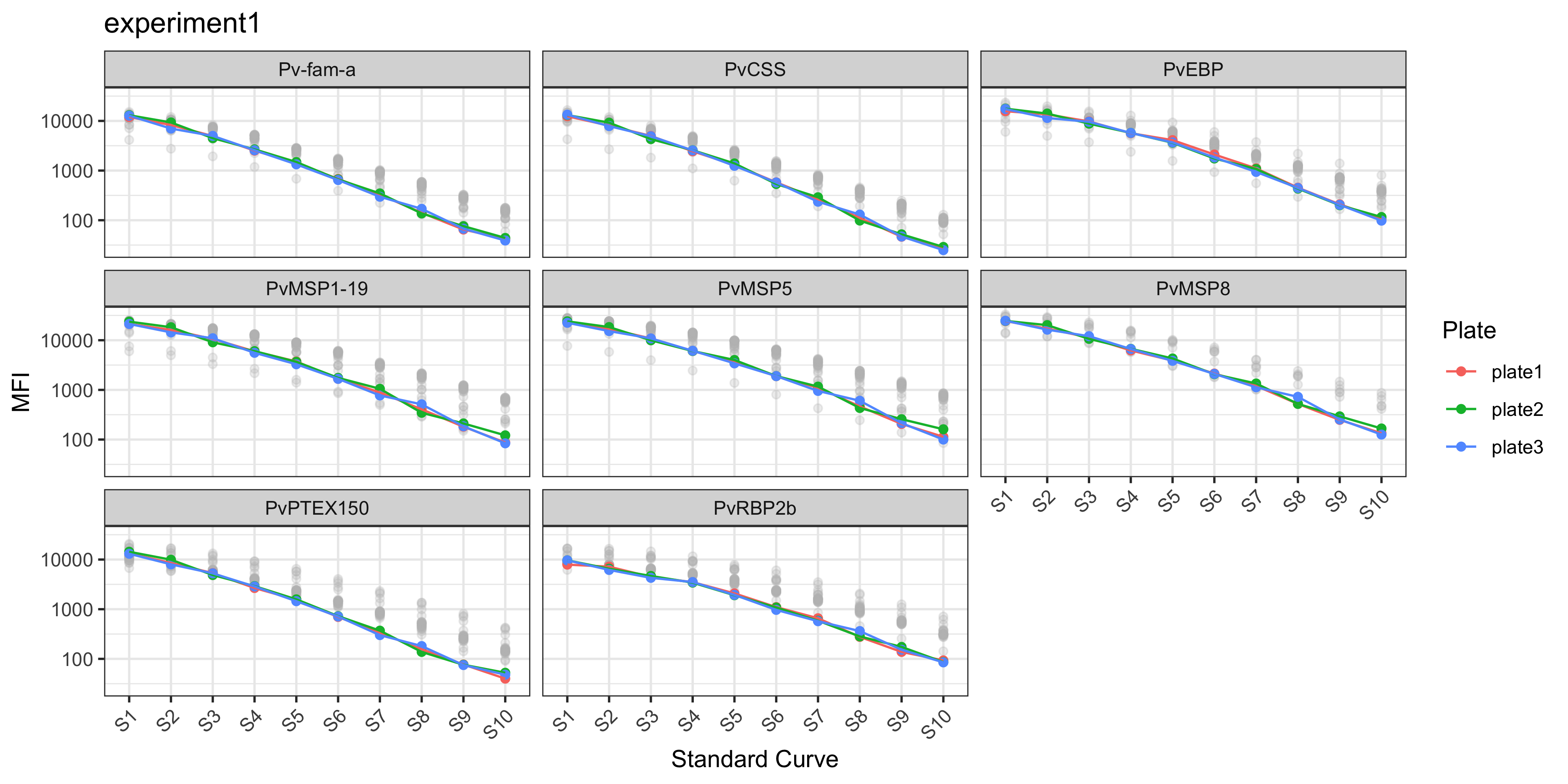
For more information on how to interrogate and visualise standard curves, see the Explore Standard Curves page.
1.1.4.2 Bead Counts QC Plot
The plotCounts() function provides a summary of the bead counts for each plate well are displayed, with blue indicating there are sufficient beads (≥15) or red when there are not enough. If any of the wells are red, they should be double-checked manually and re-run on a new plate if required.
plotCounts(qc_results, experiment_name = "experiment1")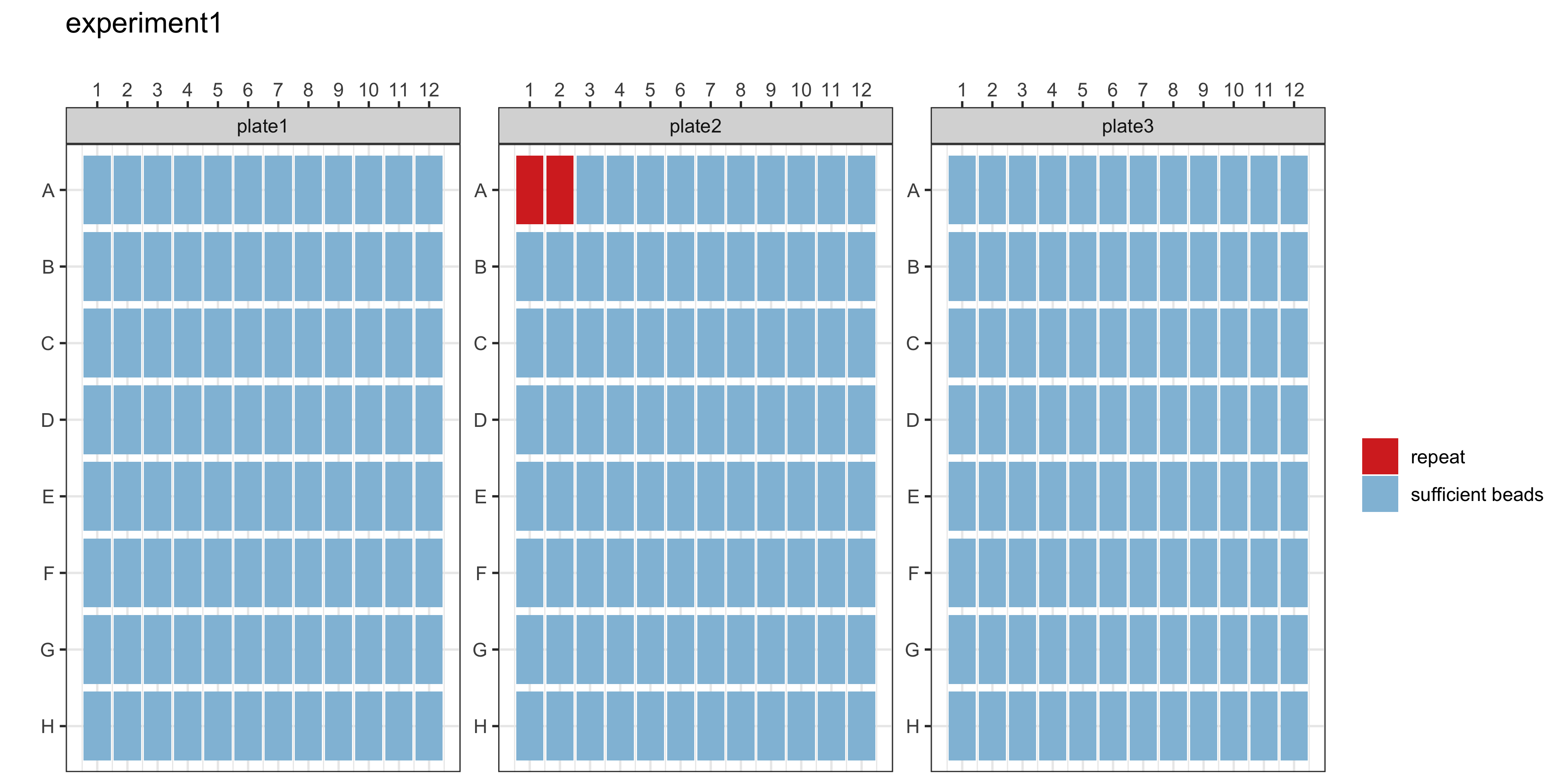
getRepeats(qc_results, plate_list)The getRepeats() function will inform you whether there are “No repeats necessary” or provide a list of samples to be re-run. In the example data, the beads in plate 2 wells A1 and A2 will need to be repeated.
| Location | SampleID | Plate | QC |
|---|---|---|---|
| A1 | Blank1 | plate2 | fail |
| A2 | Blank2 | plate2 | fail |
For more information on how to visualise these data, see the Bead Counts page.
1.1.4.3 Blanks QC Plot
The Median Fluorescent Intensity (MFI) units for each antigen is displayed for your blank samples. In general, each blank sample should have ≤50 MFI for each antigen, if they are higher they should be cross-checked manually.
plotBlanks(sero_data, experiment_name = "experiment1")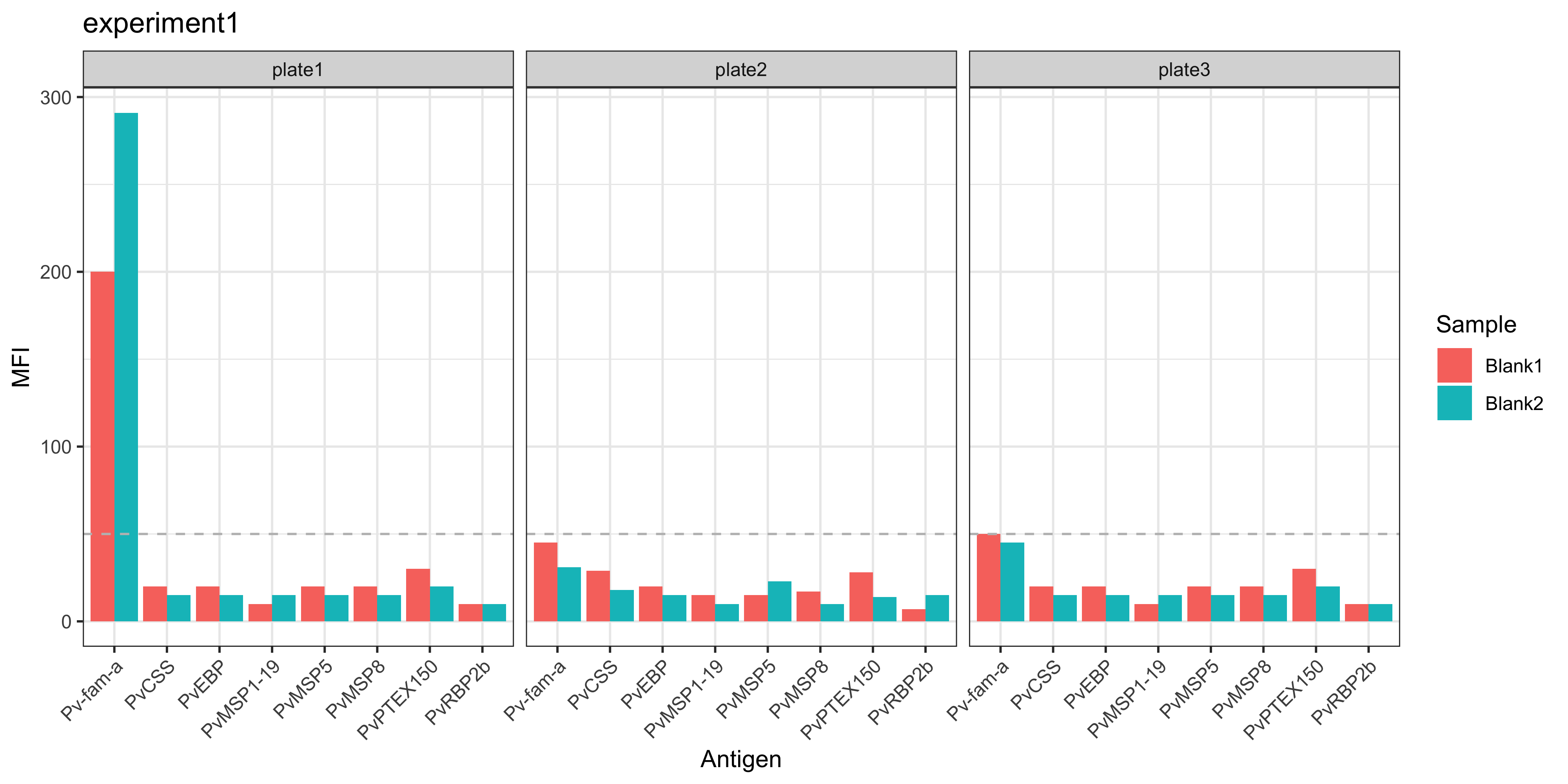
In the example data, blank samples recorded higher MFI values for LF005 on plate 1 and should be checked to confirm this is expected from the assay.
1.1.5 Step 3: MFI to RAU conversion
The automated data processing allows you to convert your Median Fluorescent Intensity (MFI) data into Relative Antibody Units (RAU) by fitting a 5-parameter logistic function to the standard curve on a per-antigen level using the MFItoRAU() function suite.
Key input variables:
sero_data,plate_list,qc_results: Previously defined variables from thereadSeroData(),readPlateLayout()andrunQC()functions.std_point: Standard Point Curve: 5 = 5-point curve, 10 = 10-point curve.
Tip
If you are using the PvSeroTAT algorithm and have used pooled positive control plasma from highly immune adults from Papua New Guinea (PNG) for your standard curve, then use the MFItoRAU() and plotModel() functions.
If you are NOT performing P. vivax serology-related work for classification, then you can also use these functions.
mfi_to_rau_output <- MFItoRAU(
  sero_data = sero_data,
  plate_list = plate_list,
  qc_results = qc_results,
  std_point = 10
)
The mfi_to_rau_output variable contains the processed MFI and RAU data for each antigen per sample. There are three data frames output from this variable:
[[1]]: Contains correct SampleID’s, well number and letters, MFI and RAU values per antigen and QC results.[[2]]: Contains correct SampleID’s, MFI and RAU values per antigen and QC results. Cleaner data frame![[3]]: Raw MFI to RAU conversion data per antigen.
If you are using the PvSeroTAT algorithm, we need to save it into a variable to use it for classification in the next step!
mfi_to_rau_output[[2]]| SampleID | Plate | PvEBP_MFI | PvEBP_Dilution | Pv-fam-a_MFI | Pv-fam-a_Dilution | PvMSP5_MFI | PvMSP5_Dilution | PvMSP1-19_MFI | PvMSP1-19_Dilution | PvMSP8_MFI | PvMSP8_Dilution | PvRBP2b_MFI | PvRBP2b_Dilution | PvPTEX150_MFI | PvPTEX150_Dilution | PvCSS_MFI | PvCSS_Dilution | Location.2 | QC_total |
|---|---|---|---|---|---|---|---|---|---|---|---|---|---|---|---|---|---|---|---|
| ABC013 | plate1 | 2712.0 | 0.0008186 | 1569.0 | 0.0013988 | 673.0 | 0.0002178 | 327.0 | 0.0001306 | 182.0 | 0.0000544 | 1068.0 | 0.0005770 | 936.0 | 0.0008127 | 223.0 | 0.0002842 | B1 | pass |
| ABC014 | plate1 | 134.0 | 0.0000506 | 378.0 | 0.0003779 | 117.0 | 0.0000420 | 197.0 | 0.0000830 | 58.0 | 0.0000195 | 465.5 | 0.0002524 | 122.0 | 0.0001229 | 93.0 | 0.0001354 | B2 | pass |
| ABC015 | plate1 | 182.0 | 0.0000672 | 209.0 | 0.0002221 | 208.0 | 0.0000724 | 374.0 | 0.0001473 | 221.5 | 0.0000657 | 463.0 | 0.0002511 | 293.0 | 0.0002780 | 868.0 | 0.0008856 | B3 | pass |
| ABC016 | plate1 | 152.0 | 0.0000569 | 229.5 | 0.0002418 | 101.0 | 0.0000364 | 89.0 | 0.0000400 | 48.0 | 0.0000195 | 591.0 | 0.0003184 | 109.0 | 0.0001103 | 110.0 | 0.0001568 | B4 | pass |
| ABC017 | plate1 | 1135.0 | 0.0003415 | 236.0 | 0.0002480 | 299.0 | 0.0001016 | 507.0 | 0.0001933 | 209.5 | 0.0000623 | 671.0 | 0.0003606 | 1665.5 | 0.0014240 | 266.0 | 0.0003288 | B5 | pass |
| ABC018 | plate1 | 174.0 | 0.0000645 | 395.0 | 0.0003930 | 175.0 | 0.0000615 | 78.0 | 0.0000353 | 70.0 | 0.0000213 | 103.0 | 0.0000486 | 294.5 | 0.0002793 | 92.0 | 0.0001341 | B6 | pass |
| ABC019 | plate1 | 421.0 | 0.0001411 | 2081.5 | 0.0018596 | 529.0 | 0.0001734 | 149.0 | 0.0000644 | 962.0 | 0.0002753 | 1441.5 | 0.0007979 | 241.0 | 0.0002324 | 282.0 | 0.0003450 | B7 | pass |
| ABC020 | plate1 | 24.0 | 0.0000195 | 49.0 | 0.0000508 | 22.0 | 0.0000195 | 13.0 | 0.0000195 | 15.5 | 0.0000195 | 14.0 | 0.0000195 | 28.0 | 0.0000258 | 17.0 | 0.0000217 | B8 | pass |
| ABC021 | plate1 | 24.0 | 0.0000195 | 45.0 | 0.0000457 | 22.0 | 0.0000195 | 13.0 | 0.0000195 | 16.0 | 0.0000195 | 13.0 | 0.0000195 | 29.0 | 0.0000269 | 17.0 | 0.0000217 | B9 | pass |
| ABC022 | plate1 | 21464.0 | 0.0200000 | 11789.0 | 0.0194273 | 2508.5 | 0.0008140 | 8001.0 | 0.0034177 | 2342.0 | 0.0006996 | 1386.0 | 0.0007638 | 1992.0 | 0.0017082 | 2927.0 | 0.0028055 | B10 | pass |
| ABC023 | plate1 | 795.0 | 0.0002469 | 6135.5 | 0.0066799 | 407.0 | 0.0001356 | 273.0 | 0.0001112 | 535.5 | 0.0001541 | 1575.0 | 0.0008822 | 8821.0 | 0.0103627 | 998.0 | 0.0010007 | B11 | pass |
| ABC024 | plate1 | 1574.0 | 0.0004662 | 348.5 | 0.0003515 | 892.0 | 0.0002854 | 288.0 | 0.0001166 | 306.0 | 0.0000897 | 590.0 | 0.0003178 | 315.0 | 0.0002971 | 366.0 | 0.0004278 | B12 | pass |
| ABC025 | plate1 | 146.0 | 0.0000548 | 408.5 | 0.0004049 | 1130.5 | 0.0003595 | 83.0 | 0.0000374 | 100.0 | 0.0000303 | 301.0 | 0.0001648 | 652.0 | 0.0005793 | 130.0 | 0.0001809 | C1 | pass |
| ABC026 | plate1 | 1330.5 | 0.0003965 | 3036.0 | 0.0027887 | 965.0 | 0.0003080 | 174.0 | 0.0000742 | 79.0 | 0.0000240 | 1090.0 | 0.0005894 | 179.0 | 0.0001765 | 92.0 | 0.0001341 | C2 | pass |
| ABC027 | plate1 | 358.0 | 0.0001225 | 4074.5 | 0.0039273 | 335.5 | 0.0001132 | 140.0 | 0.0000609 | 390.0 | 0.0001133 | 6704.0 | 0.0106491 | 8814.0 | 0.0103504 | 5627.0 | 0.0060078 | C3 | pass |
| ABC028 | plate1 | 481.0 | 0.0001585 | 1870.0 | 0.0016667 | 421.0 | 0.0001399 | 182.5 | 0.0000775 | 1777.5 | 0.0005192 | 2390.0 | 0.0014750 | 2465.0 | 0.0021348 | 411.0 | 0.0004708 | C4 | pass |
| ABC029 | plate1 | 551.0 | 0.0001785 | 1282.0 | 0.0011498 | 331.5 | 0.0001119 | 165.0 | 0.0000707 | 77.0 | 0.0000234 | 244.0 | 0.0001333 | 579.0 | 0.0005191 | 229.0 | 0.0002905 | C5 | pass |
| ABC030 | plate1 | 943.0 | 0.0002880 | 584.5 | 0.0005575 | 235.0 | 0.0000811 | 135.0 | 0.0000589 | 3017.0 | 0.0009290 | 1034.0 | 0.0005578 | 4928.0 | 0.0047092 | 7730.0 | 0.0093008 | C6 | pass |
| ABC031 | plate1 | 532.5 | 0.0001733 | 1533.0 | 0.0013673 | 315.0 | 0.0001067 | 210.0 | 0.0000879 | 2575.5 | 0.0007773 | 2903.0 | 0.0019350 | 2779.0 | 0.0024287 | 7300.0 | 0.0085588 | C7 | pass |
| ABC032 | plate1 | 768.0 | 0.0002394 | 12605.0 | 0.0200000 | 409.0 | 0.0001362 | 7632.0 | 0.0032046 | 9860.0 | 0.0042219 | 13703.0 | 0.0200000 | 5612.0 | 0.0055468 | 6383.0 | 0.0070982 | C8 | pass |
| ABC033 | plate1 | 130.0 | 0.0000491 | 239.5 | 0.0002513 | 72.0 | 0.0000261 | 64.0 | 0.0000292 | 37.0 | 0.0000195 | 156.0 | 0.0000823 | 204.0 | 0.0001992 | 49.0 | 0.0000748 | C9 | pass |
| ABC034 | plate1 | 40.0 | 0.0000195 | 60.0 | 0.0000643 | 37.0 | 0.0000195 | 25.0 | 0.0000195 | 26.5 | 0.0000195 | 23.5 | 0.0000195 | 40.0 | 0.0000391 | 27.0 | 0.0000396 | C10 | pass |
| ABC035 | plate1 | 167.0 | 0.0000621 | 605.0 | 0.0005750 | 253.0 | 0.0000869 | 329.0 | 0.0001314 | 3973.0 | 0.0012803 | 1426.5 | 0.0007887 | 803.0 | 0.0007034 | 1670.0 | 0.0016006 | C11 | pass |
| ABC036 | plate1 | 1879.0 | 0.0005559 | 4562.0 | 0.0045148 | 415.0 | 0.0001381 | 18287.0 | 0.0136007 | 11482.5 | 0.0053044 | 12031.0 | 0.0200000 | 4830.5 | 0.0045946 | 4217.0 | 0.0042141 | C12 | pass |
| ABC037 | plate1 | 256.0 | 0.0000913 | 1507.0 | 0.0013446 | 117.0 | 0.0000420 | 129.0 | 0.0000565 | 168.0 | 0.0000503 | 488.0 | 0.0002643 | 908.0 | 0.0007897 | 87.0 | 0.0001276 | D1 | pass |
| ABC038 | plate1 | 24.0 | 0.0000195 | 49.0 | 0.0000508 | 22.0 | 0.0000195 | 12.0 | 0.0000195 | 15.0 | 0.0000195 | 14.0 | 0.0000195 | 29.0 | 0.0000269 | 17.0 | 0.0000217 | D2 | pass |
| ABC039 | plate1 | 384.0 | 0.0001303 | 1708.0 | 0.0015216 | 326.0 | 0.0001102 | 1172.5 | 0.0004161 | 986.0 | 0.0002822 | 1041.0 | 0.0005617 | 299.5 | 0.0002837 | 149.0 | 0.0002031 | D3 | pass |
| ABC040 | plate1 | 210.0 | 0.0000765 | 512.0 | 0.0004952 | 221.0 | 0.0000766 | 191.0 | 0.0000807 | 89.0 | 0.0000270 | 203.0 | 0.0001100 | 410.0 | 0.0003781 | 174.5 | 0.0002318 | D4 | pass |
| ABC041 | plate1 | 351.5 | 0.0001206 | 312.0 | 0.0003185 | 165.5 | 0.0000584 | 88.0 | 0.0000396 | 66.0 | 0.0000201 | 205.0 | 0.0001112 | 200.0 | 0.0001956 | 183.0 | 0.0002412 | D5 | pass |
| ABC042 | plate1 | 1278.0 | 0.0003817 | 5810.0 | 0.0061955 | 275.0 | 0.0000940 | 230.5 | 0.0000956 | 137.0 | 0.0000413 | 2032.0 | 0.0011964 | 1762.0 | 0.0015072 | 1241.0 | 0.0012159 | D6 | pass |
| ABC043 | plate1 | 318.0 | 0.0001105 | 397.0 | 0.0003948 | 130.0 | 0.0000464 | 130.5 | 0.0000571 | 78.0 | 0.0000237 | 903.0 | 0.0004852 | 1513.5 | 0.0012942 | 325.0 | 0.0003878 | D7 | pass |
| ABC044 | plate1 | 493.5 | 0.0001621 | 2980.5 | 0.0027318 | 401.0 | 0.0001337 | 5932.5 | 0.0023109 | 3536.0 | 0.0011158 | 4699.5 | 0.0044126 | 574.0 | 0.0005149 | 5389.0 | 0.0056841 | D8 | pass |
| ABC045 | plate1 | 9686.0 | 0.0051640 | 873.0 | 0.0008022 | 333.0 | 0.0001124 | 166.0 | 0.0000711 | 791.0 | 0.0002263 | 1093.0 | 0.0005911 | 417.5 | 0.0003844 | 262.0 | 0.0003247 | D9 | pass |
| ABC046 | plate1 | 777.5 | 0.0002421 | 581.0 | 0.0005545 | 241.5 | 0.0000832 | 173.0 | 0.0000738 | 1479.5 | 0.0004278 | 899.0 | 0.0004830 | 1504.0 | 0.0012862 | 260.0 | 0.0003227 | D10 | pass |
| ABC047 | plate1 | 455.0 | 0.0001510 | 416.5 | 0.0004120 | 126.0 | 0.0000450 | 67.0 | 0.0000305 | 48.0 | 0.0000195 | 400.0 | 0.0002178 | 183.0 | 0.0001801 | 61.0 | 0.0000923 | D11 | pass |
| ABC048 | plate1 | 202.0 | 0.0000739 | 1142.0 | 0.0010301 | 137.5 | 0.0000490 | 176.0 | 0.0000750 | 204.5 | 0.0000608 | 1090.0 | 0.0005894 | 504.0 | 0.0004568 | 459.0 | 0.0005161 | D12 | pass |
| ABC049 | plate1 | 333.5 | 0.0001152 | 623.5 | 0.0005908 | 368.0 | 0.0001234 | 10430.0 | 0.0050175 | 2340.0 | 0.0006990 | 4375.0 | 0.0038303 | 1650.0 | 0.0014107 | 7801.5 | 0.0094279 | E1 | pass |
| ABC050 | plate1 | 561.0 | 0.0001814 | 7984.0 | 0.0098546 | 441.0 | 0.0001462 | 128.0 | 0.0000561 | 141.0 | 0.0000425 | 1993.0 | 0.0011679 | 2147.0 | 0.0018459 | 1502.0 | 0.0014489 | E2 | pass |
| ABC051 | plate1 | 506.5 | 0.0001659 | 340.0 | 0.0003439 | 152.5 | 0.0000540 | 147.0 | 0.0000637 | 90.0 | 0.0000273 | 600.0 | 0.0003231 | 2178.0 | 0.0018737 | 170.0 | 0.0002268 | E3 | pass |
| ABC052 | plate1 | 254.0 | 0.0000906 | 367.0 | 0.0003681 | 392.5 | 0.0001310 | 89.0 | 0.0000400 | 142.5 | 0.0000429 | 280.0 | 0.0001533 | 298.0 | 0.0002824 | 138.0 | 0.0001903 | E4 | pass |
| ABC053 | plate1 | 888.0 | 0.0002728 | 1955.0 | 0.0017437 | 438.0 | 0.0001452 | 173.0 | 0.0000738 | 507.0 | 0.0001461 | 1009.0 | 0.0005438 | 709.0 | 0.0006262 | 2040.0 | 0.0019413 | E5 | pass |
| ABC054 | plate1 | 426.0 | 0.0001426 | 1877.0 | 0.0016730 | 186.0 | 0.0000651 | 9767.0 | 0.0045446 | 15945.0 | 0.0090314 | 10073.0 | 0.0200000 | 1585.5 | 0.0013555 | 1124.0 | 0.0011122 | E6 | pass |
| ABC055 | plate1 | 5733.0 | 0.0020987 | 1301.5 | 0.0011666 | 1920.5 | 0.0006138 | 220.5 | 0.0000918 | 4833.0 | 0.0016241 | 2340.0 | 0.0014342 | 5329.0 | 0.0051931 | 2369.0 | 0.0022534 | E7 | pass |
| ABC056 | plate1 | 19092.0 | 0.0200000 | 14422.0 | 0.0200000 | 1993.0 | 0.0006379 | 12836.5 | 0.0070025 | 7426.0 | 0.0028312 | 11930.0 | 0.0200000 | 4826.0 | 0.0045893 | 3468.5 | 0.0033727 | E8 | pass |
| ABC057 | plate1 | 596.0 | 0.0001913 | 15139.0 | 0.0200000 | 371.5 | 0.0001245 | 229.0 | 0.0000950 | 535.5 | 0.0001541 | 14032.0 | 0.0200000 | 7928.5 | 0.0088615 | 1414.5 | 0.0013704 | E9 | pass |
| ABC058 | plate1 | 1028.0 | 0.0003117 | 2646.0 | 0.0023967 | 1486.0 | 0.0004721 | 292.0 | 0.0001181 | 9357.0 | 0.0039125 | 8009.0 | 0.0200000 | 3736.0 | 0.0033830 | 14370.5 | 0.0200000 | E10 | pass |
| ABC059 | plate1 | 512.0 | 0.0001674 | 4735.0 | 0.0047321 | 3408.0 | 0.0011415 | 127.5 | 0.0000559 | 191.0 | 0.0000570 | 4401.0 | 0.0038742 | 11567.0 | 0.0159341 | 2923.5 | 0.0028020 | E11 | pass |
| ABC060 | plate1 | 883.0 | 0.0002714 | 1953.0 | 0.0017419 | 755.0 | 0.0002431 | 586.0 | 0.0002202 | 122.0 | 0.0000369 | 830.0 | 0.0004455 | 425.5 | 0.0003912 | 121.0 | 0.0001702 | E12 | pass |
| ABC061 | plate1 | 977.0 | 0.0002975 | 8719.0 | 0.0113461 | 509.0 | 0.0001672 | 187.0 | 0.0000792 | 1289.0 | 0.0003708 | 12930.0 | 0.0200000 | 13891.0 | 0.0200000 | 9531.0 | 0.0128639 | F1 | pass |
| ABC062 | plate1 | 791.0 | 0.0002458 | 1944.0 | 0.0017337 | 465.0 | 0.0001536 | 216.5 | 0.0000903 | 12307.0 | 0.0059064 | 5029.0 | 0.0050893 | 4157.0 | 0.0038331 | 760.0 | 0.0007896 | F2 | pass |
| ABC063 | plate1 | 397.0 | 0.0001341 | 987.0 | 0.0008985 | 924.0 | 0.0002953 | 133.0 | 0.0000581 | 79.0 | 0.0000240 | 253.0 | 0.0001383 | 2317.5 | 0.0019997 | 1080.5 | 0.0010737 | F3 | pass |
| ABC064 | plate1 | 1111.0 | 0.0003348 | 613.0 | 0.0005818 | 357.0 | 0.0001199 | 196.0 | 0.0000826 | 8496.0 | 0.0034099 | 7914.0 | 0.0200000 | 5772.5 | 0.0057520 | 13202.0 | 0.0200000 | F4 | pass |
| ABC065 | plate1 | 956.0 | 0.0002917 | 2369.0 | 0.0021289 | 644.0 | 0.0002089 | 389.0 | 0.0001525 | 8762.0 | 0.0035616 | 9649.0 | 0.0200000 | 6437.0 | 0.0066384 | 21113.0 | 0.0200000 | F5 | pass |
| ABC066 | plate1 | 1307.0 | 0.0003899 | 20590.0 | 0.0200000 | 1335.0 | 0.0004239 | 10780.0 | 0.0052792 | 12736.0 | 0.0062343 | 25375.5 | 0.0200000 | 5493.0 | 0.0053968 | 7696.0 | 0.0092407 | F6 | pass |
| ABC067 | plate1 | 433.0 | 0.0001446 | 382.0 | 0.0003815 | 173.0 | 0.0000609 | 105.0 | 0.0000467 | 59.0 | 0.0000195 | 480.0 | 0.0002600 | 655.0 | 0.0005818 | 367.0 | 0.0004287 | F7 | pass |
| ABC068 | plate1 | 161.0 | 0.0000601 | 279.0 | 0.0002882 | 2524.5 | 0.0008196 | 105.5 | 0.0000469 | 55.0 | 0.0000195 | 307.0 | 0.0001680 | 681.5 | 0.0006036 | 472.5 | 0.0005287 | F8 | pass |
| ABC069 | plate1 | 439.0 | 0.0001464 | 732.5 | 0.0006834 | 397.0 | 0.0001324 | 2108.0 | 0.0007346 | 9692.0 | 0.0041172 | 8090.0 | 0.0200000 | 9513.0 | 0.0116240 | 7341.0 | 0.0086279 | F9 | pass |
| ABC070 | plate1 | 1837.0 | 0.0005434 | 11406.0 | 0.0182268 | 467.5 | 0.0001544 | 20011.0 | 0.0165401 | 19606.0 | 0.0130777 | 24476.5 | 0.0200000 | 5822.0 | 0.0058159 | 5127.5 | 0.0053387 | F10 | pass |
| ABC071 | plate1 | 244.0 | 0.0000875 | 1665.5 | 0.0014839 | 166.0 | 0.0000585 | 124.0 | 0.0000545 | 154.0 | 0.0000463 | 224.0 | 0.0001220 | 718.0 | 0.0006336 | 115.0 | 0.0001629 | F11 | pass |
| ABC072 | plate1 | 482.0 | 0.0001588 | 3990.5 | 0.0038297 | 388.0 | 0.0001296 | 3736.0 | 0.0013424 | 7436.0 | 0.0028364 | 7361.0 | 0.0145342 | 4111.5 | 0.0037835 | 2819.0 | 0.0026962 | F12 | pass |
| ABC073 | plate1 | 656.0 | 0.0002081 | 3103.0 | 0.0028578 | 505.0 | 0.0001660 | 14386.0 | 0.0085405 | 2343.0 | 0.0007000 | 5503.0 | 0.0062476 | 357.5 | 0.0003336 | 1215.0 | 0.0011928 | G1 | pass |
| ABC074 | plate1 | 243.0 | 0.0000872 | 568.5 | 0.0005438 | 693.0 | 0.0002240 | 141.0 | 0.0000613 | 79.0 | 0.0000240 | 339.0 | 0.0001853 | 2080.0 | 0.0017861 | 1470.0 | 0.0014202 | G2 | pass |
| ABC075 | plate1 | 1409.5 | 0.0004190 | 1123.0 | 0.0010139 | 379.0 | 0.0001268 | 153.0 | 0.0000660 | 167.5 | 0.0000502 | 1013.0 | 0.0005460 | 1553.0 | 0.0013278 | 1738.0 | 0.0016625 | G3 | pass |
| ABC076 | plate1 | 467.5 | 0.0001546 | 6741.0 | 0.0076371 | 238.0 | 0.0000821 | 174.0 | 0.0000742 | 181.0 | 0.0000541 | 6160.0 | 0.0083312 | 1660.5 | 0.0014197 | 1087.0 | 0.0010795 | G4 | pass |
| ABC077 | plate1 | 329.0 | 0.0001138 | 630.0 | 0.0005963 | 196.0 | 0.0000684 | 119.0 | 0.0000524 | 278.0 | 0.0000818 | 787.0 | 0.0004224 | 2052.5 | 0.0017617 | 2221.0 | 0.0021119 | G5 | pass |
| ABC078 | plate1 | 1122.5 | 0.0003380 | 17810.0 | 0.0200000 | 677.0 | 0.0002190 | 12254.0 | 0.0064802 | 16011.0 | 0.0090958 | 18719.0 | 0.0200000 | 3551.0 | 0.0031913 | 10222.5 | 0.0144542 | G6 | pass |
| ABC079 | plate1 | 10853.0 | 0.0066003 | 817.5 | 0.0007553 | 255.0 | 0.0000876 | 189.0 | 0.0000799 | 2247.5 | 0.0006687 | 3322.0 | 0.0023751 | 590.0 | 0.0005282 | 258.0 | 0.0003206 | G7 | pass |
| ABC080 | plate1 | 743.5 | 0.0002326 | 820.0 | 0.0007574 | 313.5 | 0.0001062 | 289.0 | 0.0001170 | 9351.5 | 0.0039092 | 7171.0 | 0.0132567 | 3062.0 | 0.0027014 | 676.5 | 0.0007149 | G8 | pass |
| ABC081 | plate1 | 723.0 | 0.0002269 | 1255.0 | 0.0011267 | 299.0 | 0.0001016 | 253.0 | 0.0001039 | 95.0 | 0.0000288 | 712.0 | 0.0003823 | 396.0 | 0.0003663 | 129.5 | 0.0001803 | G9 | pass |
| ABC082 | plate1 | 168.0 | 0.0000625 | 684.0 | 0.0006422 | 131.0 | 0.0000468 | 198.0 | 0.0000834 | 135.5 | 0.0000408 | 392.0 | 0.0002136 | 292.0 | 0.0002772 | 254.5 | 0.0003170 | G10 | pass |
| ABC083 | plate1 | 180.0 | 0.0000665 | 276.0 | 0.0002855 | 205.0 | 0.0000714 | 4646.5 | 0.0017209 | 2550.0 | 0.0007687 | 2664.5 | 0.0017113 | 724.0 | 0.0006385 | 2707.0 | 0.0025842 | G11 | pass |
| ABC084 | plate1 | 249.5 | 0.0000892 | 4104.0 | 0.0039618 | 250.0 | 0.0000860 | 96.0 | 0.0000429 | 68.0 | 0.0000207 | 1020.0 | 0.0005499 | 960.0 | 0.0008325 | 672.0 | 0.0007108 | G12 | pass |
| ABC085 | plate1 | 479.0 | 0.0001580 | 190.0 | 0.0002036 | 105.0 | 0.0000378 | 131.0 | 0.0000573 | 66.0 | 0.0000201 | 1449.0 | 0.0008026 | 1724.5 | 0.0014748 | 108.0 | 0.0001543 | H1 | pass |
| ABC086 | plate1 | 164.0 | 0.0000611 | 327.0 | 0.0003322 | 234.5 | 0.0000810 | 66.0 | 0.0000301 | 75.5 | 0.0000230 | 259.0 | 0.0001417 | 260.0 | 0.0002492 | 89.0 | 0.0001302 | H2 | pass |
| ABC087 | plate1 | 281.5 | 0.0000993 | 1794.0 | 0.0015983 | 413.0 | 0.0001374 | 75.0 | 0.0000340 | 469.5 | 0.0001356 | 802.0 | 0.0004304 | 345.0 | 0.0003229 | 744.5 | 0.0007758 | H3 | pass |
| ABC088 | plate1 | 269.0 | 0.0000954 | 1067.0 | 0.0009664 | 141.0 | 0.0000501 | 7595.0 | 0.0031836 | 14464.0 | 0.0076618 | 7592.0 | 0.0162981 | 804.5 | 0.0007047 | 467.0 | 0.0005235 | H4 | pass |
| ABC089 | plate1 | 3247.0 | 0.0010039 | 382.0 | 0.0003815 | 470.0 | 0.0001552 | 98.0 | 0.0000438 | 2319.5 | 0.0006923 | 2009.0 | 0.0011796 | 1521.0 | 0.0013006 | 1258.0 | 0.0012310 | H5 | pass |
| ABC090 | plate1 | 20593.0 | 0.0200000 | 14902.5 | 0.0200000 | 2021.0 | 0.0006473 | 10184.0 | 0.0048386 | 5805.5 | 0.0020459 | 14083.5 | 0.0200000 | 4307.5 | 0.0039987 | 3073.0 | 0.0029553 | H6 | pass |
| ABC091 | plate1 | 395.0 | 0.0001335 | 9914.0 | 0.0141030 | 211.0 | 0.0000733 | 131.5 | 0.0000575 | 325.0 | 0.0000950 | 3021.0 | 0.0020525 | 4608.0 | 0.0043372 | 1073.5 | 0.0010675 | H7 | pass |
| ABC092 | plate1 | 904.5 | 0.0002774 | 1871.0 | 0.0016676 | 793.0 | 0.0002548 | 172.0 | 0.0000734 | 6106.0 | 0.0021836 | 2093.0 | 0.0012417 | 1303.0 | 0.0011169 | 6595.5 | 0.0074226 | H8 | pass |
| ABC093 | plate1 | 323.0 | 0.0001120 | 2007.5 | 0.0017916 | 1950.0 | 0.0006236 | 106.0 | 0.0000471 | 191.0 | 0.0000570 | 2411.0 | 0.0014923 | 7377.5 | 0.0080006 | 1699.0 | 0.0016270 | H9 | pass |
| ABC094 | plate1 | 706.0 | 0.0002221 | 2087.0 | 0.0018647 | 791.0 | 0.0002542 | 169.0 | 0.0000723 | 66.0 | 0.0000201 | 990.0 | 0.0005332 | 261.0 | 0.0002501 | 65.0 | 0.0000980 | H10 | pass |
| ABC095 | plate1 | 323.0 | 0.0001120 | 4950.0 | 0.0050089 | 264.0 | 0.0000905 | 107.0 | 0.0000475 | 645.0 | 0.0001849 | 7092.0 | 0.0127660 | 8856.0 | 0.0104244 | 5330.0 | 0.0056052 | H11 | pass |
| ABC096 | plate1 | 367.0 | 0.0001252 | 1067.0 | 0.0009664 | 259.0 | 0.0000889 | 101.0 | 0.0000450 | 7423.0 | 0.0028297 | 1203.0 | 0.0006545 | 1841.5 | 0.0015762 | 335.0 | 0.0003976 | H12 | pass |
| ABC097 | plate2 | 2712.0 | 0.0009348 | 1569.0 | 0.0014012 | 673.0 | 0.0002128 | 327.0 | 0.0001217 | 182.0 | 0.0000447 | 2208.0 | 0.0015043 | 936.0 | 0.0008059 | 223.0 | 0.0002840 | B1 | pass |
| ABC098 | plate2 | 134.0 | 0.0000478 | 378.0 | 0.0003693 | 117.0 | 0.0000262 | 197.0 | 0.0000717 | 58.0 | 0.0000195 | 290.0 | 0.0001479 | 122.0 | 0.0001220 | 93.0 | 0.0001332 | B2 | pass |
| ABC099 | plate2 | 182.0 | 0.0000654 | 209.0 | 0.0002131 | 208.0 | 0.0000580 | 374.0 | 0.0001392 | 221.5 | 0.0000557 | 376.0 | 0.0001953 | 293.0 | 0.0002849 | 868.0 | 0.0008933 | B3 | pass |
| ABC100 | plate2 | 152.0 | 0.0000545 | 229.5 | 0.0002327 | 101.0 | 0.0000206 | 89.0 | 0.0000274 | 48.0 | 0.0000195 | 103.0 | 0.0000470 | 109.0 | 0.0001082 | 110.0 | 0.0001548 | B4 | pass |
| ABC101 | plate2 | 1135.0 | 0.0003780 | 236.0 | 0.0002389 | 299.0 | 0.0000892 | 507.0 | 0.0001876 | 209.5 | 0.0000524 | 650.0 | 0.0003529 | 1665.5 | 0.0013733 | 266.0 | 0.0003292 | B5 | pass |
| ABC102 | plate2 | 174.0 | 0.0000625 | 395.0 | 0.0003845 | 175.0 | 0.0000465 | 78.0 | 0.0000227 | 70.0 | 0.0000195 | 293.5 | 0.0001498 | 294.5 | 0.0002862 | 92.0 | 0.0001319 | B6 | pass |
| ABC103 | plate2 | 421.0 | 0.0001469 | 2081.5 | 0.0018613 | 529.0 | 0.0001658 | 149.0 | 0.0000524 | 962.0 | 0.0002624 | 1632.5 | 0.0010216 | 241.0 | 0.0002380 | 282.0 | 0.0003457 | B7 | pass |
| ABC104 | plate2 | 24.0 | 0.0000195 | 49.0 | 0.0000463 | 22.0 | 0.0000195 | 13.0 | 0.0000195 | 15.5 | 0.0000195 | 14.0 | 0.0000195 | 28.0 | 0.0000195 | 17.0 | 0.0000196 | B8 | pass |
| ABC105 | plate2 | 24.0 | 0.0000195 | 45.0 | 0.0000416 | 22.0 | 0.0000195 | 13.0 | 0.0000195 | 16.0 | 0.0000195 | 13.0 | 0.0000195 | 29.0 | 0.0000195 | 17.0 | 0.0000196 | B9 | pass |
| ABC106 | plate2 | 21464.0 | 0.0200000 | 11789.0 | 0.0166113 | 2508.5 | 0.0008213 | 8001.0 | 0.0033747 | 2342.0 | 0.0006723 | 9995.5 | 0.0200000 | 1992.0 | 0.0016322 | 2927.0 | 0.0027944 | B10 | pass |
| ABC107 | plate2 | 795.0 | 0.0002680 | 6135.5 | 0.0063864 | 407.0 | 0.0001255 | 273.0 | 0.0001013 | 535.5 | 0.0001431 | 7092.0 | 0.0104717 | 8821.0 | 0.0092607 | 998.0 | 0.0010093 | B11 | pass |
| ABC108 | plate2 | 1574.0 | 0.0005239 | 348.5 | 0.0003427 | 892.0 | 0.0002838 | 288.0 | 0.0001070 | 306.0 | 0.0000793 | 548.0 | 0.0002930 | 315.0 | 0.0003043 | 366.0 | 0.0004297 | B12 | pass |
| ABC109 | plate2 | 146.0 | 0.0000523 | 408.5 | 0.0003966 | 1130.5 | 0.0003609 | 83.0 | 0.0000248 | 100.0 | 0.0000219 | 443.0 | 0.0002329 | 652.0 | 0.0005830 | 130.0 | 0.0001792 | C1 | pass |
| ABC110 | plate2 | 1330.5 | 0.0004423 | 3036.0 | 0.0027736 | 965.0 | 0.0003074 | 174.0 | 0.0000626 | 79.0 | 0.0000195 | 1092.0 | 0.0006318 | 179.0 | 0.0001795 | 92.0 | 0.0001319 | C2 | pass |
| ABC111 | plate2 | 358.0 | 0.0001260 | 4074.5 | 0.0038638 | 335.5 | 0.0001015 | 140.0 | 0.0000487 | 390.0 | 0.0001027 | 7093.0 | 0.0104750 | 8814.0 | 0.0092499 | 5627.0 | 0.0058289 | C3 | pass |
| ABC112 | plate2 | 481.0 | 0.0001666 | 1870.0 | 0.0016693 | 421.0 | 0.0001301 | 182.5 | 0.0000660 | 1777.5 | 0.0004994 | 1832.0 | 0.0011805 | 2465.0 | 0.0020174 | 411.0 | 0.0004735 | C4 | pass |
| ABC113 | plate2 | 551.0 | 0.0001893 | 1282.0 | 0.0011506 | 331.5 | 0.0001002 | 165.0 | 0.0000589 | 77.0 | 0.0000195 | 244.0 | 0.0001228 | 579.0 | 0.0005246 | 229.0 | 0.0002904 | C5 | pass |
| ABC114 | plate2 | 943.0 | 0.0003157 | 584.5 | 0.0005509 | 235.0 | 0.0000673 | 135.0 | 0.0000467 | 3017.0 | 0.0008899 | 5339.0 | 0.0058959 | 4928.0 | 0.0042990 | 7730.0 | 0.0088117 | C6 | pass |
| ABC115 | plate2 | 532.5 | 0.0001833 | 1533.0 | 0.0013696 | 315.0 | 0.0000946 | 210.0 | 0.0000769 | 2575.5 | 0.0007462 | 1029.0 | 0.0005900 | 2779.0 | 0.0022809 | 7300.0 | 0.0081501 | C7 | pass |
| ABC116 | plate2 | 768.0 | 0.0002593 | 12605.0 | 0.0186107 | 409.0 | 0.0001261 | 7632.0 | 0.0031735 | 9860.0 | 0.0039078 | 7201.0 | 0.0108335 | 5612.0 | 0.0050346 | 6383.0 | 0.0068303 | C8 | pass |
| ABC117 | plate2 | 130.0 | 0.0000463 | 239.5 | 0.0002422 | 72.0 | 0.0000195 | 64.0 | 0.0000195 | 37.0 | 0.0000195 | 156.0 | 0.0000754 | 204.0 | 0.0002035 | 49.0 | 0.0000723 | C9 | pass |
| ABC118 | plate2 | 40.0 | 0.0000195 | 60.0 | 0.0000591 | 37.0 | 0.0000195 | 25.0 | 0.0000195 | 26.5 | 0.0000195 | 23.5 | 0.0000195 | 40.0 | 0.0000276 | 27.0 | 0.0000372 | C10 | pass |
| ABC119 | plate2 | 167.0 | 0.0000600 | 605.0 | 0.0005687 | 253.0 | 0.0000735 | 329.0 | 0.0001225 | 3973.0 | 0.0012195 | 2812.0 | 0.0020972 | 803.0 | 0.0007021 | 1670.0 | 0.0016095 | C11 | pass |
| ABC120 | plate2 | 1879.0 | 0.0006289 | 4562.0 | 0.0044150 | 415.0 | 0.0001281 | 18287.0 | 0.0120746 | 11482.5 | 0.0048849 | 6291.0 | 0.0081155 | 4830.5 | 0.0041982 | 4217.0 | 0.0041479 | C12 | pass |
| ABC121 | plate2 | 256.0 | 0.0000915 | 1507.0 | 0.0013467 | 117.0 | 0.0000262 | 129.0 | 0.0000442 | 168.0 | 0.0000408 | 315.0 | 0.0001616 | 908.0 | 0.0007841 | 87.0 | 0.0001254 | D1 | pass |
| ABC122 | plate2 | 24.0 | 0.0000195 | 49.0 | 0.0000463 | 22.0 | 0.0000195 | 12.0 | 0.0000195 | 15.0 | 0.0000195 | 14.0 | 0.0000195 | 29.0 | 0.0000195 | 17.0 | 0.0000196 | D2 | pass |
| ABC123 | plate2 | 384.0 | 0.0001347 | 1708.0 | 0.0015243 | 326.0 | 0.0000983 | 1172.5 | 0.0004203 | 986.0 | 0.0002692 | 902.0 | 0.0005078 | 299.5 | 0.0002907 | 149.0 | 0.0002016 | D3 | pass |
| ABC124 | plate2 | 210.0 | 0.0000754 | 512.0 | 0.0004878 | 221.0 | 0.0000625 | 191.0 | 0.0000694 | 89.0 | 0.0000195 | 398.0 | 0.0002076 | 410.0 | 0.0003858 | 174.5 | 0.0002308 | D4 | pass |
| ABC125 | plate2 | 351.5 | 0.0001239 | 312.0 | 0.0003095 | 165.5 | 0.0000432 | 88.0 | 0.0000270 | 66.0 | 0.0000195 | 174.0 | 0.0000850 | 200.0 | 0.0001997 | 183.0 | 0.0002403 | D5 | pass |
| ABC126 | plate2 | 1278.0 | 0.0004249 | 5810.0 | 0.0059530 | 275.0 | 0.0000810 | 230.5 | 0.0000849 | 137.0 | 0.0000322 | 1903.7 | 0.0012398 | 1762.0 | 0.0014493 | 1241.0 | 0.0012254 | D6 | pass |
| ABC127 | plate2 | 318.0 | 0.0001126 | 397.0 | 0.0003863 | 130.0 | 0.0000308 | 130.5 | 0.0000448 | 78.0 | 0.0000195 | 492.1 | 0.0002608 | 1513.5 | 0.0012542 | 325.0 | 0.0003892 | D7 | pass |
| ABC128 | plate2 | 493.5 | 0.0001707 | 2980.5 | 0.0027183 | 401.0 | 0.0001235 | 5932.5 | 0.0023171 | 3536.0 | 0.0010656 | 4699.5 | 0.0046875 | 574.0 | 0.0005205 | 5389.0 | 0.0055288 | D8 | pass |
| ABC129 | plate2 | 9686.0 | 0.0053458 | 873.0 | 0.0007990 | 333.0 | 0.0001007 | 166.0 | 0.0000593 | 791.0 | 0.0002143 | 653.0 | 0.0003546 | 417.5 | 0.0003921 | 262.0 | 0.0003251 | D9 | pass |
| ABC130 | plate2 | 777.5 | 0.0002623 | 581.0 | 0.0005479 | 241.5 | 0.0000695 | 173.0 | 0.0000622 | 1479.5 | 0.0004112 | 439.0 | 0.0002307 | 1504.0 | 0.0012468 | 260.0 | 0.0003230 | D10 | pass |
| ABC131 | plate2 | 455.0 | 0.0001581 | 416.5 | 0.0004037 | 126.0 | 0.0000293 | 67.0 | 0.0000195 | 48.0 | 0.0000195 | 143.0 | 0.0000684 | 183.0 | 0.0001834 | 61.0 | 0.0000898 | D11 | pass |
| ABC132 | plate2 | 202.0 | 0.0000726 | 1142.0 | 0.0010298 | 137.5 | 0.0000334 | 176.0 | 0.0000634 | 204.5 | 0.0000510 | 210.0 | 0.0001044 | 504.0 | 0.0004637 | 459.0 | 0.0005193 | D12 | pass |
| ABC133 | plate2 | 333.5 | 0.0001178 | 623.5 | 0.0005847 | 368.0 | 0.0001124 | 10430.0 | 0.0048535 | 2340.0 | 0.0006717 | 4375.0 | 0.0041471 | 1650.0 | 0.0013611 | 7801.5 | 0.0089245 | E1 | pass |
| ABC134 | plate2 | 561.0 | 0.0001926 | 7984.0 | 0.0091295 | 441.0 | 0.0001367 | 128.0 | 0.0000438 | 141.0 | 0.0000333 | 431.0 | 0.0002261 | 2147.0 | 0.0017570 | 1502.0 | 0.0014584 | E2 | pass |
| ABC135 | plate2 | 506.5 | 0.0001749 | 340.0 | 0.0003351 | 152.5 | 0.0000386 | 147.0 | 0.0000516 | 90.0 | 0.0000195 | 299.0 | 0.0001528 | 2178.0 | 0.0017821 | 170.0 | 0.0002257 | E3 | pass |
| ABC136 | plate2 | 254.0 | 0.0000908 | 367.0 | 0.0003594 | 392.5 | 0.0001206 | 89.0 | 0.0000274 | 142.5 | 0.0000337 | 323.5 | 0.0001663 | 298.0 | 0.0002893 | 138.0 | 0.0001887 | E4 | pass |
| ABC137 | plate2 | 888.0 | 0.0002979 | 1955.0 | 0.0017461 | 438.0 | 0.0001358 | 173.0 | 0.0000622 | 507.0 | 0.0001351 | 829.0 | 0.0004619 | 709.0 | 0.0006282 | 2040.0 | 0.0019473 | E5 | pass |
| ABC138 | plate2 | 426.0 | 0.0001486 | 1877.0 | 0.0016756 | 186.0 | 0.0000503 | 9767.0 | 0.0044219 | 15945.0 | 0.0082439 | 10073.0 | 0.0200000 | 1585.5 | 0.0013105 | 1124.0 | 0.0011213 | E6 | pass |
| ABC139 | plate2 | 5733.0 | 0.0023603 | 1301.5 | 0.0011675 | 1920.5 | 0.0006207 | 220.5 | 0.0000810 | 4833.0 | 0.0015390 | 3718.0 | 0.0031830 | 5329.0 | 0.0047242 | 2369.0 | 0.0022548 | E7 | pass |
| ABC140 | plate2 | 19092.0 | 0.0200000 | 14422.0 | 0.0200000 | 1993.0 | 0.0006450 | 12836.5 | 0.0066197 | 7426.0 | 0.0026465 | 14663.0 | 0.0200000 | 4826.0 | 0.0041936 | 3468.5 | 0.0033433 | E8 | pass |
| ABC141 | plate2 | 596.0 | 0.0002039 | 15139.0 | 0.0200000 | 371.5 | 0.0001136 | 229.0 | 0.0000843 | 535.5 | 0.0001431 | 9105.0 | 0.0192940 | 7928.5 | 0.0079416 | 1414.5 | 0.0013801 | E9 | pass |
| ABC142 | plate2 | 1028.0 | 0.0003432 | 2646.0 | 0.0023913 | 1486.0 | 0.0004767 | 292.0 | 0.0001085 | 9357.0 | 0.0036279 | 7769.5 | 0.0129060 | 3736.0 | 0.0031296 | 14370.5 | 0.0200000 | E10 | pass |
| ABC143 | plate2 | 512.0 | 0.0001767 | 4735.0 | 0.0046170 | 3408.0 | 0.0011443 | 127.5 | 0.0000436 | 191.0 | 0.0000472 | 2401.0 | 0.0016835 | 11567.0 | 0.0141915 | 2923.5 | 0.0027910 | E11 | pass |
| ABC144 | plate2 | 883.0 | 0.0002963 | 1953.0 | 0.0017442 | 755.0 | 0.0002394 | 586.0 | 0.0002158 | 122.0 | 0.0000280 | 398.0 | 0.0002076 | 425.5 | 0.0003988 | 121.0 | 0.0001683 | E12 | pass |
| ABC145 | plate2 | 977.0 | 0.0003267 | 8719.0 | 0.0103665 | 509.0 | 0.0001592 | 187.0 | 0.0000678 | 1289.0 | 0.0003558 | 6039.5 | 0.0074739 | 13891.0 | 0.0196656 | 9531.0 | 0.0119146 | F1 | pass |
| ABC146 | plate2 | 791.0 | 0.0002667 | 1944.0 | 0.0017361 | 465.0 | 0.0001447 | 216.5 | 0.0000794 | 12307.0 | 0.0054275 | 3907.0 | 0.0034437 | 4157.0 | 0.0035274 | 760.0 | 0.0007964 | F2 | pass |
| ABC147 | plate2 | 397.0 | 0.0001390 | 987.0 | 0.0008966 | 924.0 | 0.0002941 | 133.0 | 0.0000459 | 79.0 | 0.0000195 | 253.0 | 0.0001277 | 2317.5 | 0.0018959 | 1080.5 | 0.0010827 | F3 | pass |
| ABC148 | plate2 | 1111.0 | 0.0003702 | 613.0 | 0.0005756 | 357.0 | 0.0001087 | 196.0 | 0.0000713 | 8496.0 | 0.0031725 | 914.0 | 0.0005155 | 5772.5 | 0.0052146 | 13202.0 | 0.0200000 | F4 | pass |
| ABC149 | plate2 | 956.0 | 0.0003199 | 2369.0 | 0.0021279 | 644.0 | 0.0002034 | 389.0 | 0.0001447 | 8762.0 | 0.0033101 | 7649.0 | 0.0124392 | 6437.0 | 0.0059919 | 21113.0 | 0.0200000 | F5 | pass |
| ABC150 | plate2 | 1307.0 | 0.0004345 | 20590.0 | 0.0200000 | 1335.0 | 0.0004274 | 10780.0 | 0.0050904 | 12736.0 | 0.0057228 | 9375.5 | 0.0200000 | 5493.0 | 0.0049030 | 7696.0 | 0.0087583 | F6 | pass |
| ABC151 | plate2 | 433.0 | 0.0001509 | 382.0 | 0.0003729 | 173.0 | 0.0000458 | 105.0 | 0.0000342 | 59.0 | 0.0000195 | 599.0 | 0.0003227 | 655.0 | 0.0005854 | 367.0 | 0.0004307 | F7 | pass |
| ABC152 | plate2 | 161.0 | 0.0000578 | 279.0 | 0.0002791 | 2524.5 | 0.0008269 | 105.5 | 0.0000344 | 55.0 | 0.0000195 | 491.0 | 0.0002602 | 681.5 | 0.0006064 | 472.5 | 0.0005321 | F8 | pass |
| ABC153 | plate2 | 439.0 | 0.0001528 | 732.5 | 0.0006785 | 397.0 | 0.0001221 | 2108.0 | 0.0007488 | 9692.0 | 0.0038132 | 8115.0 | 0.0143344 | 9513.0 | 0.0103716 | 7341.0 | 0.0082119 | F9 | pass |
| ABC154 | plate2 | 1837.0 | 0.0006142 | 11406.0 | 0.0157263 | 467.5 | 0.0001455 | 20011.0 | 0.0143419 | 19606.0 | 0.0119087 | 9476.5 | 0.0200000 | 5822.0 | 0.0052708 | 5127.5 | 0.0052070 | F10 | pass |
| ABC155 | plate2 | 244.0 | 0.0000873 | 1665.5 | 0.0014865 | 166.0 | 0.0000434 | 124.0 | 0.0000421 | 154.0 | 0.0000369 | 224.0 | 0.0001120 | 718.0 | 0.0006353 | 115.0 | 0.0001610 | F11 | pass |
| ABC156 | plate2 | 482.0 | 0.0001669 | 3990.5 | 0.0037715 | 388.0 | 0.0001191 | 3736.0 | 0.0013636 | 7436.0 | 0.0026512 | 2361.0 | 0.0016456 | 4111.5 | 0.0034836 | 2819.0 | 0.0026880 | F12 | pass |
| ABC157 | plate2 | 656.0 | 0.0002232 | 3103.0 | 0.0028407 | 505.0 | 0.0001579 | 14386.0 | 0.0079437 | 2343.0 | 0.0006727 | 803.0 | 0.0004457 | 357.5 | 0.0003412 | 1215.0 | 0.0012023 | G1 | pass |
| ABC158 | plate2 | 243.0 | 0.0000870 | 568.5 | 0.0005370 | 693.0 | 0.0002193 | 141.0 | 0.0000492 | 79.0 | 0.0000195 | 995.0 | 0.0005677 | 2080.0 | 0.0017029 | 1470.0 | 0.0014297 | G2 | pass |
| ABC159 | plate2 | 1409.5 | 0.0004686 | 1123.0 | 0.0010134 | 379.0 | 0.0001161 | 153.0 | 0.0000541 | 167.5 | 0.0000407 | 480.5 | 0.0002542 | 1553.0 | 0.0012851 | 1738.0 | 0.0016711 | G3 | pass |
| ABC160 | plate2 | 467.5 | 0.0001622 | 6741.0 | 0.0072305 | 238.0 | 0.0000683 | 174.0 | 0.0000626 | 181.0 | 0.0000444 | 904.5 | 0.0005094 | 1660.5 | 0.0013693 | 1087.0 | 0.0010884 | G4 | pass |
| ABC161 | plate2 | 329.0 | 0.0001163 | 630.0 | 0.0005903 | 196.0 | 0.0000538 | 119.0 | 0.0000401 | 278.0 | 0.0000715 | 321.0 | 0.0001649 | 2052.5 | 0.0016808 | 2221.0 | 0.0021156 | G5 | pass |
| ABC162 | plate2 | 1122.5 | 0.0003739 | 17810.0 | 0.0200000 | 677.0 | 0.0002141 | 12254.0 | 0.0061616 | 16011.0 | 0.0083020 | 18719.0 | 0.0200000 | 3551.0 | 0.0029598 | 10222.5 | 0.0132637 | G6 | pass |
| ABC163 | plate2 | 10853.0 | 0.0065838 | 817.5 | 0.0007514 | 255.0 | 0.0000742 | 189.0 | 0.0000686 | 2247.5 | 0.0006428 | 479.0 | 0.0002533 | 590.0 | 0.0005334 | 258.0 | 0.0003209 | G7 | pass |
| ABC164 | plate2 | 743.5 | 0.0002514 | 820.0 | 0.0007536 | 313.5 | 0.0000941 | 289.0 | 0.0001074 | 9351.5 | 0.0036249 | 771.0 | 0.0004260 | 3062.0 | 0.0025244 | 676.5 | 0.0007208 | G8 | pass |
| ABC165 | plate2 | 723.0 | 0.0002448 | 1255.0 | 0.0011273 | 299.0 | 0.0000892 | 253.0 | 0.0000936 | 95.0 | 0.0000205 | 803.0 | 0.0004457 | 396.0 | 0.0003740 | 129.5 | 0.0001786 | G9 | pass |
| ABC166 | plate2 | 168.0 | 0.0000603 | 684.0 | 0.0006368 | 131.0 | 0.0000311 | 198.0 | 0.0000721 | 135.5 | 0.0000317 | 329.0 | 0.0001693 | 292.0 | 0.0002840 | 254.5 | 0.0003173 | G10 | pass |
| ABC167 | plate2 | 180.0 | 0.0000647 | 276.0 | 0.0002764 | 205.0 | 0.0000569 | 4646.5 | 0.0017398 | 2550.0 | 0.0007381 | 2664.5 | 0.0019436 | 724.0 | 0.0006400 | 2707.0 | 0.0025787 | G11 | pass |
| ABC168 | plate2 | 249.5 | 0.0000892 | 4104.0 | 0.0038964 | 250.0 | 0.0000724 | 96.0 | 0.0000304 | 68.0 | 0.0000195 | 702.0 | 0.0003840 | 960.0 | 0.0008245 | 672.0 | 0.0007167 | G12 | pass |
| ABC169 | plate2 | 479.0 | 0.0001659 | 190.0 | 0.0001947 | 105.0 | 0.0000220 | 131.0 | 0.0000450 | 66.0 | 0.0000195 | 809.0 | 0.0004494 | 1724.5 | 0.0014197 | 108.0 | 0.0001523 | H1 | pass |
| ABC170 | plate2 | 164.0 | 0.0000589 | 327.0 | 0.0003232 | 234.5 | 0.0000671 | 66.0 | 0.0000195 | 75.5 | 0.0000195 | 259.0 | 0.0001310 | 260.0 | 0.0002553 | 89.0 | 0.0001280 | H2 | pass |
| ABC171 | plate2 | 281.5 | 0.0001002 | 1794.0 | 0.0016010 | 413.0 | 0.0001274 | 75.0 | 0.0000214 | 469.5 | 0.0001247 | 388.0 | 0.0002020 | 345.0 | 0.0003304 | 744.5 | 0.0007824 | H3 | pass |
| ABC172 | plate2 | 269.0 | 0.0000959 | 1067.0 | 0.0009653 | 141.0 | 0.0000346 | 7595.0 | 0.0031536 | 14464.0 | 0.0070089 | 7592.0 | 0.0122238 | 804.5 | 0.0007033 | 467.0 | 0.0005269 | H4 | pass |
| ABC173 | plate2 | 3247.0 | 0.0011483 | 382.0 | 0.0003729 | 470.0 | 0.0001463 | 98.0 | 0.0000312 | 2319.5 | 0.0006653 | 1904.5 | 0.0012405 | 1521.0 | 0.0012601 | 1258.0 | 0.0012405 | H5 | pass |
| ABC174 | plate2 | 20593.0 | 0.0200000 | 14902.5 | 0.0200000 | 2021.0 | 0.0006544 | 10184.0 | 0.0046908 | 5805.5 | 0.0019280 | 9083.5 | 0.0191706 | 4307.5 | 0.0036735 | 3073.0 | 0.0029399 | H6 | pass |
| ABC175 | plate2 | 395.0 | 0.0001383 | 9914.0 | 0.0125777 | 211.0 | 0.0000590 | 131.5 | 0.0000452 | 325.0 | 0.0000846 | 6791.0 | 0.0095263 | 4608.0 | 0.0039717 | 1073.5 | 0.0010764 | H7 | pass |
| ABC176 | plate2 | 904.5 | 0.0003032 | 1871.0 | 0.0016702 | 793.0 | 0.0002517 | 172.0 | 0.0000618 | 6106.0 | 0.0020544 | 5444.0 | 0.0061144 | 1303.0 | 0.0010904 | 6595.5 | 0.0071256 | H8 | pass |
| ABC177 | plate2 | 323.0 | 0.0001143 | 2007.5 | 0.0017938 | 1950.0 | 0.0006306 | 106.0 | 0.0000346 | 191.0 | 0.0000472 | 1411.0 | 0.0008549 | 7377.5 | 0.0071862 | 1699.0 | 0.0016358 | H9 | pass |
| ABC178 | plate2 | 706.0 | 0.0002393 | 2087.0 | 0.0018664 | 791.0 | 0.0002511 | 169.0 | 0.0000605 | 66.0 | 0.0000195 | 899.0 | 0.0005059 | 261.0 | 0.0002562 | 65.0 | 0.0000955 | H10 | pass |
| ABC179 | plate2 | 323.0 | 0.0001143 | 4950.0 | 0.0048730 | 264.0 | 0.0000772 | 107.0 | 0.0000350 | 645.0 | 0.0001735 | 5201.0 | 0.0056178 | 8856.0 | 0.0093150 | 5330.0 | 0.0054555 | H11 | pass |
| ABC180 | plate2 | 367.0 | 0.0001290 | 1067.0 | 0.0009653 | 259.0 | 0.0000755 | 101.0 | 0.0000325 | 7423.0 | 0.0026450 | 2494.0 | 0.0017733 | 1841.5 | 0.0015123 | 335.0 | 0.0003991 | H12 | pass |
| ABC181 | plate3 | 2712.0 | 0.0009247 | 1569.0 | 0.0014825 | 673.0 | 0.0002101 | 327.0 | 0.0001255 | 182.0 | 0.0000532 | 593.0 | 0.0003089 | 936.0 | 0.0008214 | 223.0 | 0.0002777 | B1 | pass |
| ABC182 | plate3 | 134.0 | 0.0000527 | 378.0 | 0.0003718 | 117.0 | 0.0000437 | 197.0 | 0.0000800 | 58.0 | 0.0000195 | 128.0 | 0.0000604 | 122.0 | 0.0001195 | 93.0 | 0.0001316 | B2 | pass |
| ABC183 | plate3 | 182.0 | 0.0000700 | 209.0 | 0.0002132 | 208.0 | 0.0000719 | 374.0 | 0.0001416 | 221.5 | 0.0000635 | 348.0 | 0.0001722 | 293.0 | 0.0002804 | 868.0 | 0.0009003 | B3 | pass |
| ABC184 | plate3 | 152.0 | 0.0000593 | 229.5 | 0.0002328 | 101.0 | 0.0000385 | 89.0 | 0.0000401 | 48.0 | 0.0000195 | 180.0 | 0.0000860 | 109.0 | 0.0001063 | 110.0 | 0.0001521 | B4 | pass |
| ABC185 | plate3 | 1135.0 | 0.0003741 | 236.0 | 0.0002390 | 299.0 | 0.0000992 | 507.0 | 0.0001870 | 209.5 | 0.0000604 | 650.0 | 0.0003426 | 1665.5 | 0.0014322 | 266.0 | 0.0003225 | B5 | pass |
| ABC186 | plate3 | 174.0 | 0.0000671 | 395.0 | 0.0003875 | 175.0 | 0.0000618 | 78.0 | 0.0000357 | 70.0 | 0.0000229 | 293.5 | 0.0001436 | 294.5 | 0.0002817 | 92.0 | 0.0001304 | B6 | pass |
| ABC187 | plate3 | 421.0 | 0.0001492 | 2081.5 | 0.0019939 | 529.0 | 0.0001673 | 149.0 | 0.0000627 | 962.0 | 0.0002567 | 532.5 | 0.0002739 | 241.0 | 0.0002334 | 282.0 | 0.0003389 | B7 | pass |
| ABC188 | plate3 | 24.0 | 0.0000195 | 49.0 | 0.0000513 | 22.0 | 0.0000195 | 13.0 | 0.0000195 | 15.5 | 0.0000195 | 14.0 | 0.0000195 | 28.0 | 0.0000195 | 17.0 | 0.0000272 | B8 | pass |
| ABC189 | plate3 | 24.0 | 0.0000195 | 45.0 | 0.0000469 | 22.0 | 0.0000195 | 13.0 | 0.0000195 | 16.0 | 0.0000195 | 13.0 | 0.0000195 | 29.0 | 0.0000195 | 17.0 | 0.0000272 | B9 | pass |
| ABC190 | plate3 | 21464.0 | 0.0200000 | 11789.0 | 0.0188708 | 2508.5 | 0.0008167 | 8001.0 | 0.0038346 | 2342.0 | 0.0006614 | 9995.5 | 0.0200000 | 1992.0 | 0.0017157 | 2927.0 | 0.0029083 | B10 | pass |
| ABC191 | plate3 | 795.0 | 0.0002668 | 6135.5 | 0.0071560 | 407.0 | 0.0001312 | 273.0 | 0.0001068 | 535.5 | 0.0001443 | 12560.0 | 0.0200000 | 8821.0 | 0.0106456 | 998.0 | 0.0010214 | B11 | pass |
| ABC192 | plate3 | 1574.0 | 0.0005171 | 348.5 | 0.0003445 | 892.0 | 0.0002761 | 288.0 | 0.0001120 | 306.0 | 0.0000853 | 2060.0 | 0.0014281 | 315.0 | 0.0002999 | 366.0 | 0.0004233 | B12 | pass |
| ABC193 | plate3 | 146.0 | 0.0000571 | 408.5 | 0.0003999 | 1130.5 | 0.0003497 | 83.0 | 0.0000377 | 100.0 | 0.0000313 | 201.0 | 0.0000965 | 652.0 | 0.0005866 | 130.0 | 0.0001755 | C1 | pass |
| ABC194 | plate3 | 1330.5 | 0.0004370 | 3036.0 | 0.0030211 | 965.0 | 0.0002985 | 174.0 | 0.0000718 | 79.0 | 0.0000255 | 709.0 | 0.0003783 | 179.0 | 0.0001754 | 92.0 | 0.0001304 | C2 | pass |
| ABC195 | plate3 | 358.0 | 0.0001289 | 4074.5 | 0.0042619 | 335.5 | 0.0001101 | 140.0 | 0.0000594 | 390.0 | 0.0001069 | 5769.5 | 0.0074520 | 8814.0 | 0.0106324 | 5627.0 | 0.0060911 | C3 | pass |
| ABC196 | plate3 | 481.0 | 0.0001683 | 1870.0 | 0.0017797 | 421.0 | 0.0001354 | 182.5 | 0.0000748 | 1777.5 | 0.0004877 | 1845.0 | 0.0012294 | 2465.0 | 0.0021415 | 411.0 | 0.0004676 | C4 | pass |
| ABC197 | plate3 | 551.0 | 0.0001904 | 1282.0 | 0.0012069 | 331.5 | 0.0001089 | 165.0 | 0.0000685 | 77.0 | 0.0000249 | 244.0 | 0.0001182 | 579.0 | 0.0005258 | 229.0 | 0.0002840 | C5 | pass |
| ABC198 | plate3 | 943.0 | 0.0003132 | 584.5 | 0.0005611 | 235.0 | 0.0000801 | 135.0 | 0.0000575 | 3017.0 | 0.0008846 | 5339.0 | 0.0064372 | 4928.0 | 0.0047368 | 7730.0 | 0.0091448 | C6 | pass |
| ABC199 | plate3 | 532.5 | 0.0001845 | 1533.0 | 0.0014476 | 315.0 | 0.0001040 | 210.0 | 0.0000847 | 2575.5 | 0.0007367 | 4592.5 | 0.0049079 | 2779.0 | 0.0024354 | 7300.0 | 0.0084741 | C7 | pass |
| ABC200 | plate3 | 768.0 | 0.0002583 | 12605.0 | 0.0200000 | 409.0 | 0.0001318 | 7632.0 | 0.0035905 | 9860.0 | 0.0041857 | 9340.5 | 0.0200000 | 5612.0 | 0.0055933 | 6383.0 | 0.0071250 | C8 | pass |
| ABC201 | plate3 | 130.0 | 0.0000512 | 239.5 | 0.0002423 | 72.0 | 0.0000289 | 64.0 | 0.0000301 | 37.0 | 0.0000195 | 156.0 | 0.0000741 | 204.0 | 0.0001991 | 49.0 | 0.0000748 | C9 | pass |
| ABC202 | plate3 | 40.0 | 0.0000195 | 60.0 | 0.0000633 | 37.0 | 0.0000195 | 25.0 | 0.0000195 | 26.5 | 0.0000195 | 23.5 | 0.0000195 | 40.0 | 0.0000313 | 27.0 | 0.0000430 | C10 | pass |
| ABC203 | plate3 | 167.0 | 0.0000646 | 605.0 | 0.0005798 | 253.0 | 0.0000855 | 329.0 | 0.0001262 | 3973.0 | 0.0012300 | 1412.0 | 0.0008669 | 803.0 | 0.0007116 | 1670.0 | 0.0016533 | C11 | pass |
| ABC204 | plate3 | 1879.0 | 0.0006206 | 4562.0 | 0.0048924 | 415.0 | 0.0001336 | 18287.0 | 0.0144135 | 11482.5 | 0.0052803 | 5816.0 | 0.0075679 | 4830.5 | 0.0046200 | 4217.0 | 0.0043363 | C12 | pass |
| ABC205 | plate3 | 256.0 | 0.0000953 | 1507.0 | 0.0014224 | 117.0 | 0.0000437 | 129.0 | 0.0000553 | 168.0 | 0.0000495 | 315.0 | 0.0001548 | 908.0 | 0.0007983 | 87.0 | 0.0001242 | D1 | pass |
| ABC206 | plate3 | 24.0 | 0.0000195 | 49.0 | 0.0000513 | 22.0 | 0.0000195 | 12.0 | 0.0000195 | 15.0 | 0.0000195 | 14.0 | 0.0000195 | 29.0 | 0.0000195 | 17.0 | 0.0000272 | D2 | pass |
| ABC207 | plate3 | 384.0 | 0.0001373 | 1708.0 | 0.0016187 | 326.0 | 0.0001072 | 1172.5 | 0.0004162 | 986.0 | 0.0002631 | 1562.0 | 0.0009869 | 299.5 | 0.0002862 | 149.0 | 0.0001972 | D3 | pass |
| ABC208 | plate3 | 210.0 | 0.0000797 | 512.0 | 0.0004948 | 221.0 | 0.0000758 | 191.0 | 0.0000779 | 89.0 | 0.0000282 | 293.5 | 0.0001436 | 410.0 | 0.0003827 | 174.5 | 0.0002255 | D4 | pass |
| ABC209 | plate3 | 351.5 | 0.0001268 | 312.0 | 0.0003105 | 165.5 | 0.0000589 | 88.0 | 0.0000397 | 66.0 | 0.0000218 | 218.5 | 0.0001053 | 200.0 | 0.0001953 | 183.0 | 0.0002348 | D5 | pass |
| ABC210 | plate3 | 1278.0 | 0.0004200 | 5810.0 | 0.0066577 | 275.0 | 0.0000921 | 230.5 | 0.0000919 | 137.0 | 0.0000413 | 729.5 | 0.0003908 | 1762.0 | 0.0015152 | 1241.0 | 0.0012481 | D6 | pass |
| ABC211 | plate3 | 318.0 | 0.0001159 | 397.0 | 0.0003893 | 130.0 | 0.0000478 | 130.5 | 0.0000558 | 78.0 | 0.0000252 | 440.0 | 0.0002220 | 1513.5 | 0.0013027 | 325.0 | 0.0003825 | D7 | pass |
| ABC212 | plate3 | 493.5 | 0.0001722 | 2980.5 | 0.0029585 | 401.0 | 0.0001295 | 5932.5 | 0.0025618 | 3536.0 | 0.0010678 | 4699.5 | 0.0051104 | 574.0 | 0.0005216 | 5389.0 | 0.0057795 | D8 | pass |
| ABC213 | plate3 | 9686.0 | 0.0056594 | 873.0 | 0.0008252 | 333.0 | 0.0001093 | 166.0 | 0.0000689 | 791.0 | 0.0002110 | 621.0 | 0.0003253 | 417.5 | 0.0003892 | 262.0 | 0.0003184 | D9 | pass |
| ABC214 | plate3 | 777.5 | 0.0002613 | 581.0 | 0.0005579 | 241.5 | 0.0000820 | 173.0 | 0.0000714 | 1479.5 | 0.0004006 | 1037.5 | 0.0005918 | 1504.0 | 0.0012947 | 260.0 | 0.0003163 | D10 | pass |
| ABC215 | plate3 | 455.0 | 0.0001600 | 416.5 | 0.0004073 | 126.0 | 0.0000465 | 67.0 | 0.0000313 | 48.0 | 0.0000195 | 270.0 | 0.0001315 | 183.0 | 0.0001793 | 61.0 | 0.0000910 | D11 | pass |
| ABC216 | plate3 | 202.0 | 0.0000769 | 1142.0 | 0.0010750 | 137.5 | 0.0000502 | 176.0 | 0.0000725 | 204.5 | 0.0000591 | 897.0 | 0.0004973 | 504.0 | 0.0004628 | 459.0 | 0.0005142 | D12 | pass |
| ABC217 | plate3 | 333.5 | 0.0001210 | 623.5 | 0.0005967 | 368.0 | 0.0001197 | 10430.0 | 0.0056405 | 2340.0 | 0.0006608 | 4375.0 | 0.0045122 | 1650.0 | 0.0014189 | 7801.5 | 0.0092588 | E1 | pass |
| ABC218 | plate3 | 561.0 | 0.0001935 | 7984.0 | 0.0103116 | 441.0 | 0.0001413 | 128.0 | 0.0000549 | 141.0 | 0.0000424 | 2119.5 | 0.0014854 | 2147.0 | 0.0018531 | 1502.0 | 0.0014936 | E2 | pass |
| ABC219 | plate3 | 506.5 | 0.0001763 | 340.0 | 0.0003366 | 152.5 | 0.0000549 | 147.0 | 0.0000619 | 90.0 | 0.0000285 | 399.0 | 0.0001996 | 2178.0 | 0.0018809 | 170.0 | 0.0002206 | E3 | pass |
| ABC220 | plate3 | 254.0 | 0.0000947 | 367.0 | 0.0003616 | 392.5 | 0.0001269 | 89.0 | 0.0000401 | 142.5 | 0.0000428 | 323.5 | 0.0001593 | 298.0 | 0.0002848 | 138.0 | 0.0001847 | E4 | pass |
| ABC221 | plate3 | 888.0 | 0.0002959 | 1955.0 | 0.0018652 | 438.0 | 0.0001404 | 173.0 | 0.0000714 | 507.0 | 0.0001369 | 1584.0 | 0.0010050 | 709.0 | 0.0006339 | 2040.0 | 0.0020108 | E5 | pass |
| ABC222 | plate3 | 426.0 | 0.0001508 | 1877.0 | 0.0017867 | 186.0 | 0.0000652 | 9767.0 | 0.0051118 | 15945.0 | 0.0090345 | 10073.0 | 0.0200000 | 1585.5 | 0.0013639 | 1124.0 | 0.0011388 | E6 | pass |
| ABC223 | plate3 | 5733.0 | 0.0023881 | 1301.5 | 0.0012254 | 1920.5 | 0.0006082 | 220.5 | 0.0000884 | 4833.0 | 0.0015710 | 3718.0 | 0.0034396 | 5329.0 | 0.0052308 | 2369.0 | 0.0023366 | E7 | pass |
| ABC224 | plate3 | 19092.0 | 0.0200000 | 14422.0 | 0.0200000 | 1993.0 | 0.0006331 | 12836.5 | 0.0078070 | 7426.0 | 0.0027812 | 8663.0 | 0.0176802 | 4826.0 | 0.0046146 | 3468.5 | 0.0034887 | E8 | pass |
| ABC225 | plate3 | 596.0 | 0.0002045 | 15139.0 | 0.0200000 | 371.5 | 0.0001207 | 229.0 | 0.0000914 | 535.5 | 0.0001443 | 8105.0 | 0.0151456 | 7928.5 | 0.0090475 | 1414.5 | 0.0014110 | E9 | pass |
| ABC226 | plate3 | 1028.0 | 0.0003401 | 2646.0 | 0.0025890 | 1486.0 | 0.0004631 | 292.0 | 0.0001134 | 9357.0 | 0.0038727 | 7769.5 | 0.0137702 | 3736.0 | 0.0033933 | 14370.5 | 0.0200000 | E10 | pass |
| ABC227 | plate3 | 512.0 | 0.0001781 | 4735.0 | 0.0051239 | 3408.0 | 0.0011638 | 127.5 | 0.0000547 | 191.0 | 0.0000556 | 901.0 | 0.0005000 | 11567.0 | 0.0167561 | 2923.5 | 0.0029046 | E11 | pass |
| ABC228 | plate3 | 883.0 | 0.0002944 | 1953.0 | 0.0018632 | 755.0 | 0.0002347 | 586.0 | 0.0002138 | 122.0 | 0.0000373 | 529.0 | 0.0002719 | 425.5 | 0.0003960 | 121.0 | 0.0001651 | E12 | pass |
| ABC229 | plate3 | 977.0 | 0.0003240 | 8719.0 | 0.0117330 | 509.0 | 0.0001614 | 187.0 | 0.0000765 | 1289.0 | 0.0003466 | 5039.5 | 0.0057903 | 13891.0 | 0.0200000 | 9531.0 | 0.0122411 | F1 | pass |
| ABC230 | plate3 | 791.0 | 0.0002655 | 1944.0 | 0.0018541 | 465.0 | 0.0001484 | 216.5 | 0.0000870 | 12307.0 | 0.0058888 | 8907.0 | 0.0188942 | 4157.0 | 0.0038475 | 760.0 | 0.0007994 | F2 | pass |
| ABC231 | plate3 | 397.0 | 0.0001415 | 987.0 | 0.0009305 | 924.0 | 0.0002859 | 133.0 | 0.0000568 | 79.0 | 0.0000255 | 253.0 | 0.0001228 | 2317.5 | 0.0020067 | 1080.5 | 0.0010982 | F3 | pass |
| ABC232 | plate3 | 1111.0 | 0.0003664 | 613.0 | 0.0005871 | 357.0 | 0.0001164 | 196.0 | 0.0000797 | 8496.0 | 0.0033650 | 7914.0 | 0.0143496 | 5772.5 | 0.0058041 | 13202.0 | 0.0200000 | F4 | pass |
| ABC233 | plate3 | 956.0 | 0.0003173 | 2369.0 | 0.0022926 | 644.0 | 0.0002015 | 389.0 | 0.0001468 | 8762.0 | 0.0035181 | 4649.0 | 0.0050142 | 6437.0 | 0.0067194 | 21113.0 | 0.0200000 | F5 | pass |
| ABC234 | plate3 | 1307.0 | 0.0004294 | 20590.0 | 0.0200000 | 1335.0 | 0.0004144 | 10780.0 | 0.0059310 | 12736.0 | 0.0062199 | 7375.5 | 0.0122844 | 5493.0 | 0.0054394 | 7696.0 | 0.0090909 | F6 | pass |
| ABC235 | plate3 | 433.0 | 0.0001530 | 382.0 | 0.0003755 | 173.0 | 0.0000612 | 105.0 | 0.0000462 | 59.0 | 0.0000198 | 599.0 | 0.0003124 | 655.0 | 0.0005891 | 367.0 | 0.0004243 | F7 | pass |
| ABC236 | plate3 | 161.0 | 0.0000625 | 279.0 | 0.0002796 | 2524.5 | 0.0008226 | 105.5 | 0.0000464 | 55.0 | 0.0000195 | 491.0 | 0.0002504 | 681.5 | 0.0006111 | 472.5 | 0.0005273 | F8 | pass |
| ABC237 | plate3 | 439.0 | 0.0001549 | 732.5 | 0.0006963 | 397.0 | 0.0001283 | 2108.0 | 0.0007615 | 9692.0 | 0.0040798 | 6115.0 | 0.0083445 | 9513.0 | 0.0120045 | 7341.0 | 0.0085370 | F9 | pass |
| ABC238 | plate3 | 1837.0 | 0.0006061 | 11406.0 | 0.0178640 | 467.5 | 0.0001491 | 20011.0 | 0.0170964 | 19606.0 | 0.0130628 | 5476.5 | 0.0067501 | 5822.0 | 0.0058699 | 5127.5 | 0.0054445 | F10 | pass |
| ABC239 | plate3 | 244.0 | 0.0000913 | 1665.5 | 0.0015769 | 166.0 | 0.0000590 | 124.0 | 0.0000534 | 154.0 | 0.0000458 | 224.0 | 0.0001080 | 718.0 | 0.0006414 | 115.0 | 0.0001580 | F11 | pass |
| ABC240 | plate3 | 482.0 | 0.0001686 | 3990.5 | 0.0041565 | 388.0 | 0.0001256 | 3736.0 | 0.0014467 | 7436.0 | 0.0027864 | 3361.0 | 0.0029278 | 4111.5 | 0.0037974 | 2819.0 | 0.0027956 | F12 | pass |
| ABC241 | plate3 | 656.0 | 0.0002233 | 3103.0 | 0.0030971 | 505.0 | 0.0001602 | 14386.0 | 0.0094265 | 2343.0 | 0.0006617 | 2503.0 | 0.0018792 | 357.5 | 0.0003373 | 1215.0 | 0.0012238 | G1 | pass |
| ABC242 | plate3 | 243.0 | 0.0000909 | 568.5 | 0.0005465 | 693.0 | 0.0002161 | 141.0 | 0.0000597 | 79.0 | 0.0000255 | 1295.0 | 0.0007772 | 2080.0 | 0.0017935 | 1470.0 | 0.0014634 | G2 | pass |
| ABC243 | plate3 | 1409.5 | 0.0004628 | 1123.0 | 0.0010572 | 379.0 | 0.0001230 | 153.0 | 0.0000641 | 167.5 | 0.0000494 | 1280.5 | 0.0007663 | 1553.0 | 0.0013362 | 1738.0 | 0.0017184 | G3 | pass |
| ABC244 | plate3 | 467.5 | 0.0001640 | 6741.0 | 0.0081271 | 238.0 | 0.0000810 | 174.0 | 0.0000718 | 181.0 | 0.0000529 | 1804.5 | 0.0011934 | 1660.5 | 0.0014279 | 1087.0 | 0.0011043 | G4 | pass |
| ABC245 | plate3 | 329.0 | 0.0001195 | 630.0 | 0.0006026 | 196.0 | 0.0000682 | 119.0 | 0.0000515 | 278.0 | 0.0000781 | 223.0 | 0.0001075 | 2052.5 | 0.0017691 | 2221.0 | 0.0021891 | G5 | pass |
| ABC246 | plate3 | 1122.5 | 0.0003701 | 17810.0 | 0.0200000 | 677.0 | 0.0002113 | 12254.0 | 0.0072453 | 16011.0 | 0.0090991 | 3142.0 | 0.0026367 | 3551.0 | 0.0032003 | 10222.5 | 0.0135633 | G6 | pass |
| ABC247 | plate3 | 10853.0 | 0.0070873 | 817.5 | 0.0007742 | 255.0 | 0.0000861 | 189.0 | 0.0000772 | 2247.5 | 0.0006315 | 1023.0 | 0.0005818 | 590.0 | 0.0005350 | 258.0 | 0.0003143 | G7 | pass |
| ABC248 | plate3 | 743.5 | 0.0002507 | 820.0 | 0.0007765 | 313.5 | 0.0001035 | 289.0 | 0.0001124 | 9351.5 | 0.0038694 | 873.0 | 0.0004817 | 3062.0 | 0.0027085 | 676.5 | 0.0007211 | G8 | pass |
| ABC249 | plate3 | 723.0 | 0.0002443 | 1255.0 | 0.0011814 | 299.0 | 0.0000992 | 253.0 | 0.0000998 | 95.0 | 0.0000299 | 203.0 | 0.0000975 | 396.0 | 0.0003707 | 129.5 | 0.0001749 | G9 | pass |
| ABC250 | plate3 | 168.0 | 0.0000650 | 684.0 | 0.0006519 | 131.0 | 0.0000481 | 198.0 | 0.0000804 | 135.5 | 0.0000409 | 223.4 | 0.0001077 | 292.0 | 0.0002795 | 254.5 | 0.0003106 | G10 | pass |
| ABC251 | plate3 | 180.0 | 0.0000692 | 276.0 | 0.0002768 | 205.0 | 0.0000710 | 4646.5 | 0.0018811 | 2550.0 | 0.0007284 | 664.5 | 0.0003513 | 724.0 | 0.0006463 | 2707.0 | 0.0026798 | G11 | pass |
| ABC252 | plate3 | 249.5 | 0.0000931 | 4104.0 | 0.0042992 | 250.0 | 0.0000846 | 96.0 | 0.0000428 | 68.0 | 0.0000223 | 563.0 | 0.0002914 | 960.0 | 0.0008412 | 672.0 | 0.0007169 | G12 | pass |
| ABC253 | plate3 | 479.0 | 0.0001676 | 190.0 | 0.0001949 | 105.0 | 0.0000398 | 131.0 | 0.0000560 | 66.0 | 0.0000218 | 406.0 | 0.0002034 | 1724.5 | 0.0014829 | 108.0 | 0.0001497 | H1 | pass |
| ABC254 | plate3 | 164.0 | 0.0000636 | 327.0 | 0.0003245 | 234.5 | 0.0000799 | 66.0 | 0.0000309 | 75.5 | 0.0000245 | 259.0 | 0.0001258 | 260.0 | 0.0002507 | 89.0 | 0.0001267 | H2 | pass |
| ABC255 | plate3 | 281.5 | 0.0001038 | 1794.0 | 0.0017038 | 413.0 | 0.0001330 | 75.0 | 0.0000345 | 469.5 | 0.0001273 | 530.5 | 0.0002727 | 345.0 | 0.0003263 | 744.5 | 0.0007849 | H3 | pass |
| ABC256 | plate3 | 269.0 | 0.0000997 | 1067.0 | 0.0010049 | 141.0 | 0.0000513 | 7595.0 | 0.0035665 | 14464.0 | 0.0076590 | 7592.0 | 0.0130842 | 804.5 | 0.0007129 | 467.0 | 0.0005220 | H4 | pass |
| ABC257 | plate3 | 3247.0 | 0.0011392 | 382.0 | 0.0003755 | 470.0 | 0.0001499 | 98.0 | 0.0000435 | 2319.5 | 0.0006543 | 2304.5 | 0.0016700 | 1521.0 | 0.0013091 | 1258.0 | 0.0012640 | H5 | pass |
| ABC258 | plate3 | 20593.0 | 0.0200000 | 14902.5 | 0.0200000 | 2021.0 | 0.0006428 | 10184.0 | 0.0054411 | 5805.5 | 0.0019921 | 14083.5 | 0.0200000 | 4307.5 | 0.0040151 | 3073.0 | 0.0030622 | H6 | pass |
| ABC259 | plate3 | 395.0 | 0.0001409 | 9914.0 | 0.0142686 | 211.0 | 0.0000728 | 131.5 | 0.0000562 | 325.0 | 0.0000902 | 2791.0 | 0.0022043 | 4608.0 | 0.0043583 | 1073.5 | 0.0010917 | H7 | pass |
| ABC260 | plate3 | 904.5 | 0.0003011 | 1871.0 | 0.0017807 | 793.0 | 0.0002461 | 172.0 | 0.0000711 | 6106.0 | 0.0021301 | 744.0 | 0.0003998 | 1303.0 | 0.0011257 | 6595.5 | 0.0074281 | H8 | pass |
| ABC261 | plate3 | 323.0 | 0.0001175 | 2007.5 | 0.0019184 | 1950.0 | 0.0006183 | 106.0 | 0.0000466 | 191.0 | 0.0000556 | 2411.0 | 0.0017808 | 7377.5 | 0.0081404 | 1699.0 | 0.0016810 | H9 | pass |
| ABC262 | plate3 | 706.0 | 0.0002389 | 2087.0 | 0.0019995 | 791.0 | 0.0002455 | 169.0 | 0.0000700 | 66.0 | 0.0000218 | 412.0 | 0.0002066 | 261.0 | 0.0002516 | 65.0 | 0.0000963 | H10 | pass |
| ABC263 | plate3 | 323.0 | 0.0001175 | 4950.0 | 0.0054174 | 264.0 | 0.0000888 | 107.0 | 0.0000470 | 645.0 | 0.0001727 | 2381.0 | 0.0017492 | 8856.0 | 0.0107118 | 5330.0 | 0.0057032 | H11 | pass |
| ABC264 | plate3 | 367.0 | 0.0001318 | 1067.0 | 0.0010049 | 259.0 | 0.0000873 | 101.0 | 0.0000447 | 7423.0 | 0.0027796 | 1494.0 | 0.0009318 | 1841.5 | 0.0015840 | 335.0 | 0.0003925 | H12 | pass |
The results from this log-log conversion should look relatively linear for each antigen and can be plotted using the plotModel() function suite.
plotModel(mfi_to_rau_output, sero_data)
#> $`1`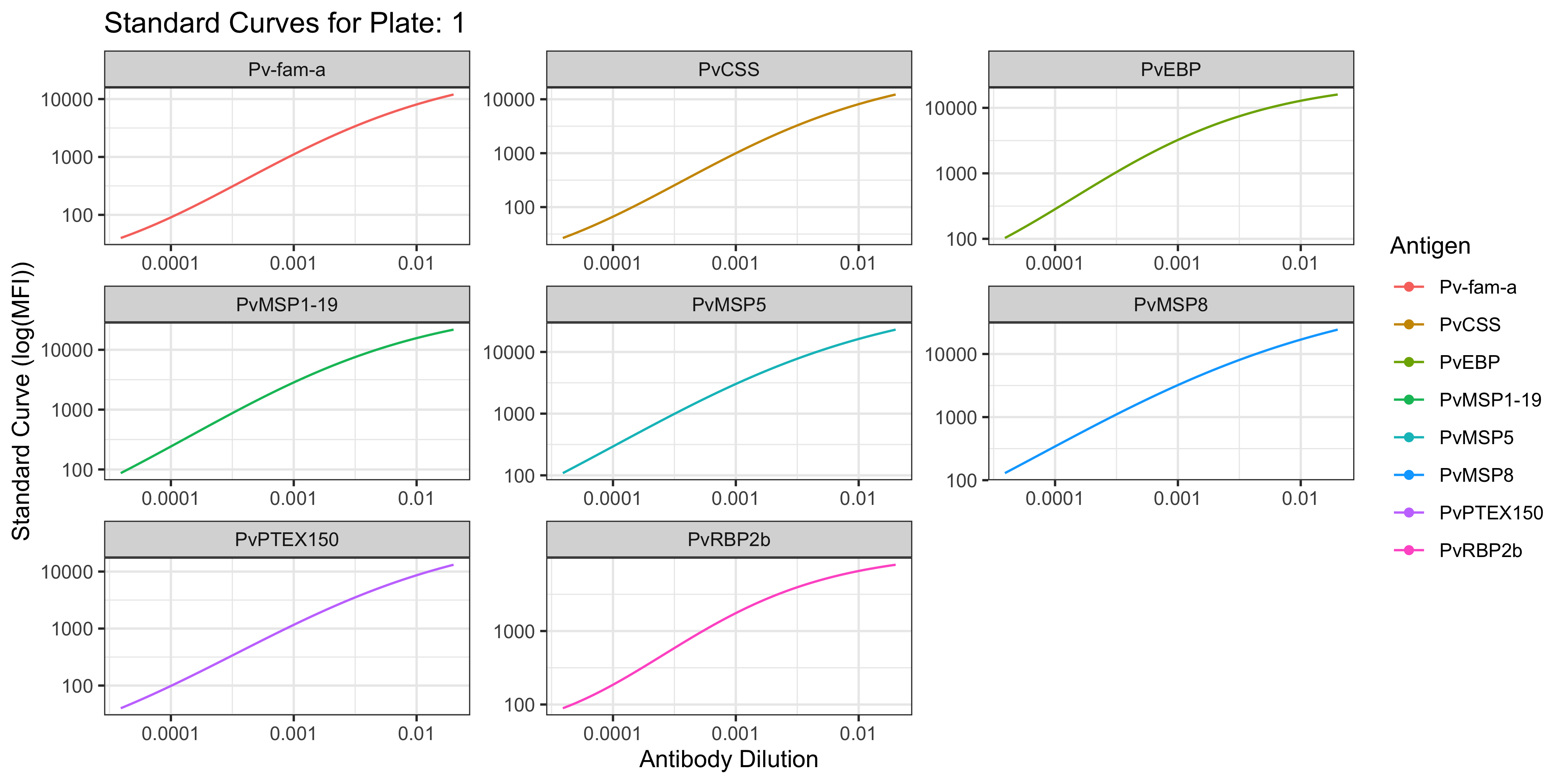
#>
#> $`2`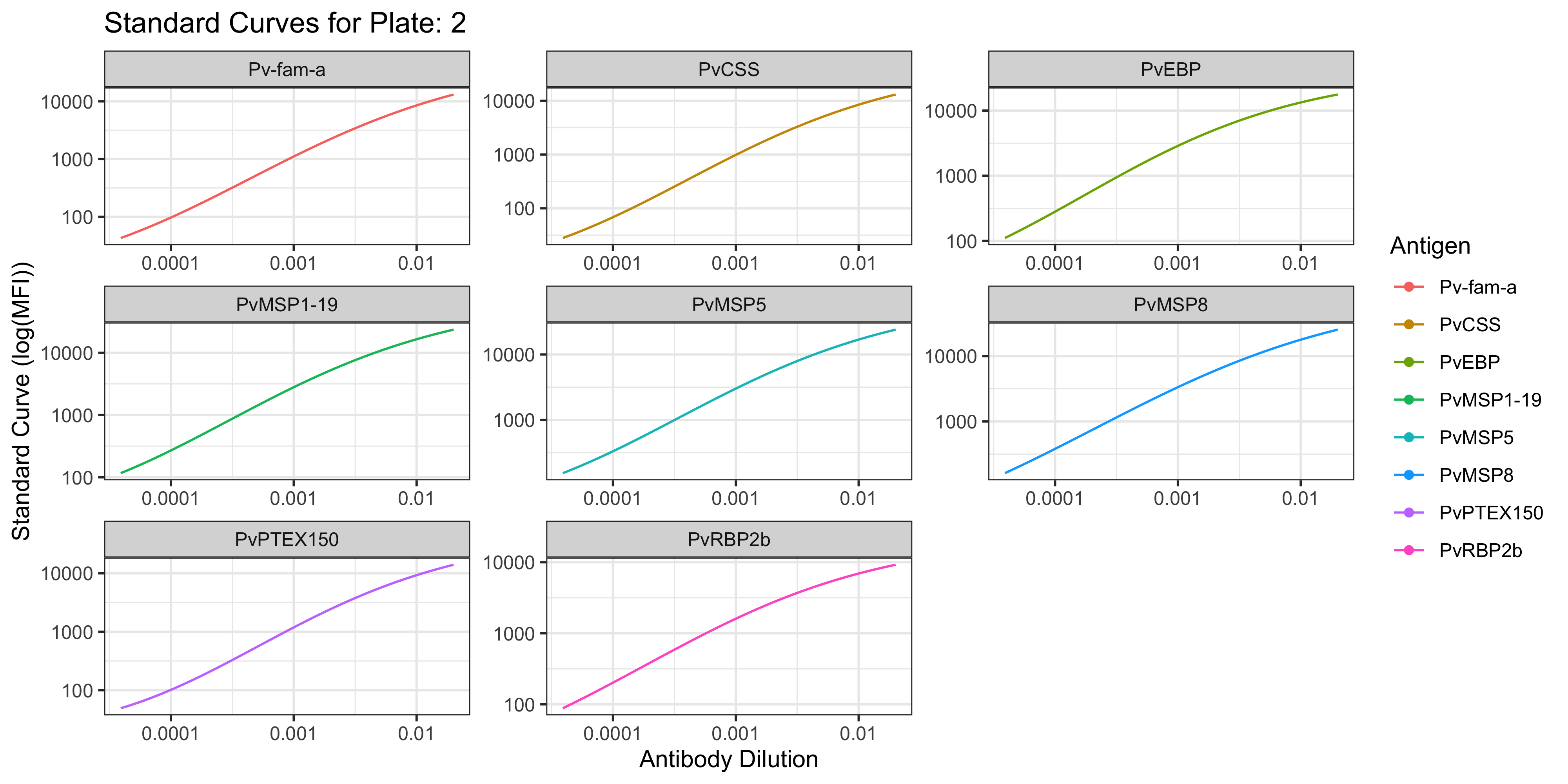
#>
#> $`3`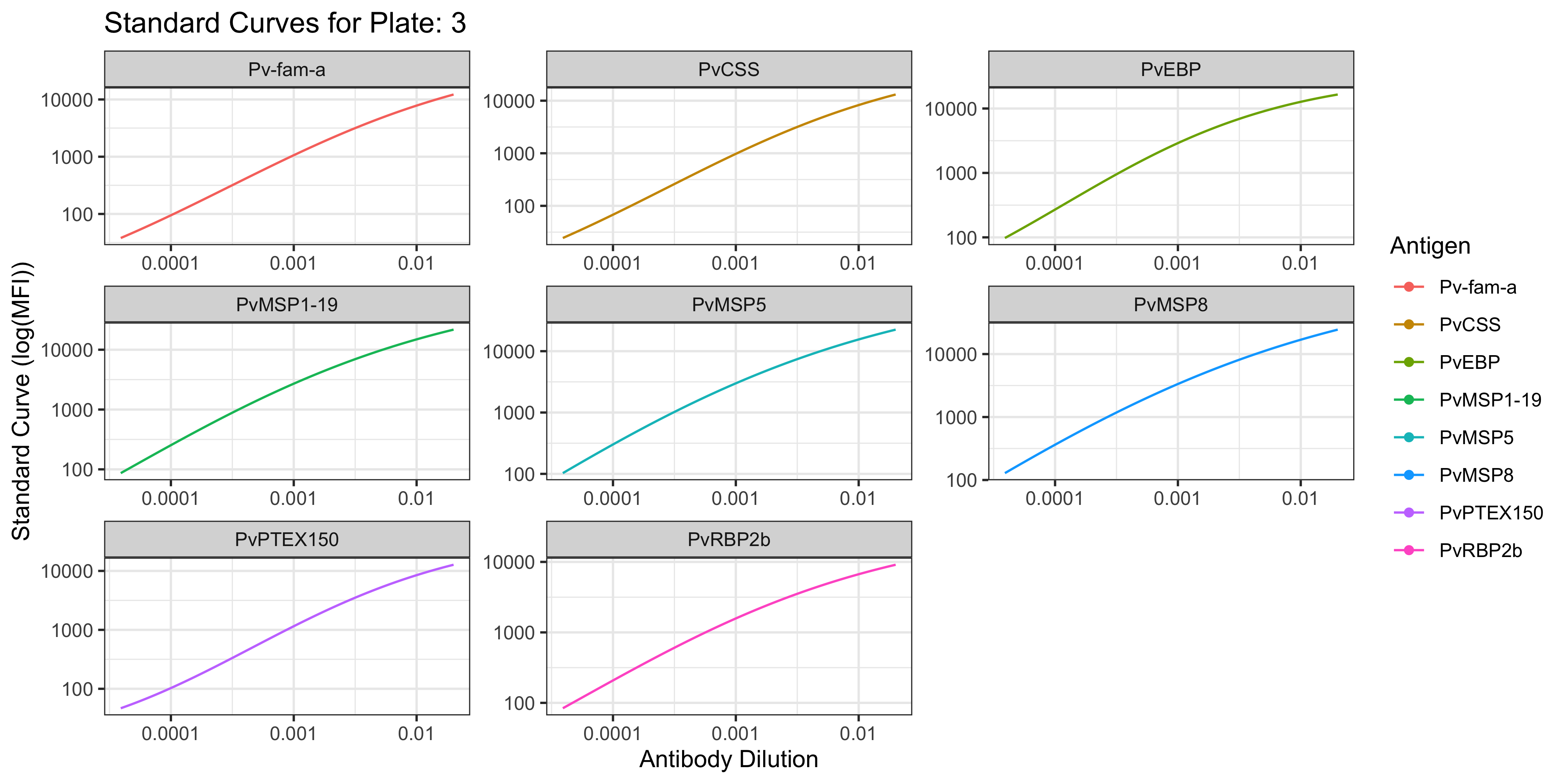
Tip
If you are performing the PvSeroTAT algorithm and have used pooled positive control plasma from highly immune adults from Ethiopia (ETH) for your standard curve, then use the MFItoRAU_Adj() and plotModel_Adj() functions.
mfi_to_rau_output <- MFItoRAU_Adj(
  sero_data,
  plate_list,
  qc_results,
  std_point = 10
)
plotModel_Adj(mfi_to_rau_output, sero_data)
#> $plate1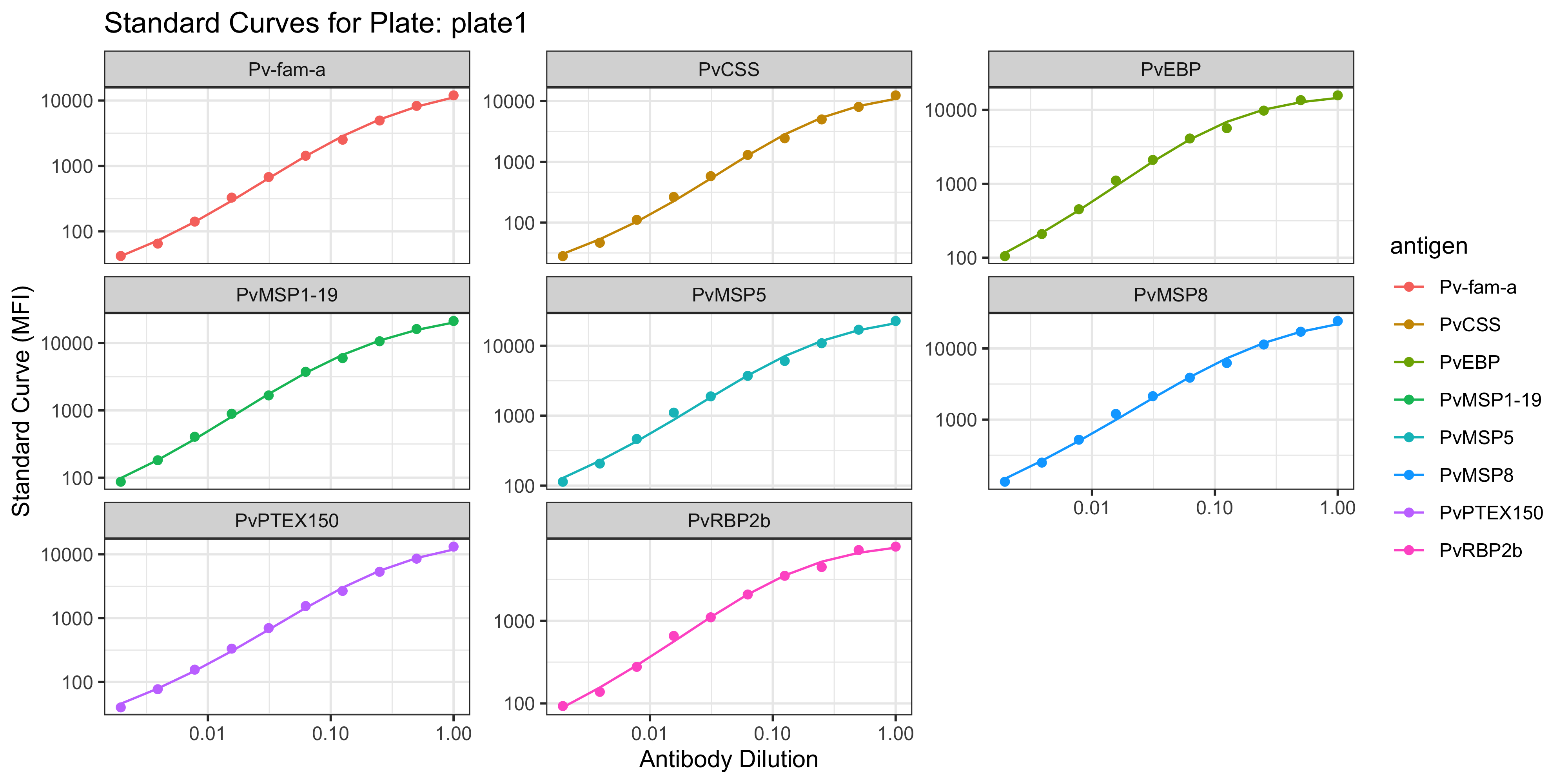
#>
#> $plate2
#>
#> $plate3
For more information on how to visualise MFI and RAU data, see the MFI and RAU plots page.
1.1.6 Step 4: Classification
This final function classifies samples as recently exposed within the last nine months (“seropositive”) or not (“seronegative”).
The algorithm_type is only “antibody_model”, which is also written by default.
The sens_spec can be:
- “balanced” (default)
- “90% specificity”
TipWhich sensitivity/specificity threshold do I use?
The balanced sensitivity / specificity is when both metrics are at their highest and correspond to 81% each.
High specificity with lower sensitivity is suited for surveillance settings and aims to correctly identify non-carriers and minimise treatment of uninfected individual, while the impact of false negatives can be mitigated by increasing survey size.
classifyResults_output <- classifyResults(
  mfi_to_rau_output,
  algorithm_type = "antibody_model",
  sens_spec = "balanced",
  qc_results
)
The results from the classification are displayed in a table. The exposure status (seropositive/seronegative) is displayed for each sample.
To form an educated guess about the seropositivity/exposure status for your samples, take into consideration all relevant epidemiological information that you may have available to you (e.g. time since possible exposure, timing of sampling with respect to incidence of P. vivax infections/cases) and explore the results using the classifier/s.
classifyResults_output| SampleID | Plate | QC_total | PvEBP | Pv-fam-a | PvMSP5 | PvMSP1-19 | PvMSP8 | PvPTEX150 | PvCSS | PvRBP2b | pred_class_max |
|---|---|---|---|---|---|---|---|---|---|---|---|
| ABC013 | plate1 | pass | 0.0003339 | 0.0015045 | 0.0002163 | 0.0014567 | 0.0000195 | 0.0001591 | 0.0000772 | 0.0003714 | seropositive |
| ABC097 | plate2 | pass | 0.0004324 | 0.0015615 | 0.0001944 | 0.0013373 | 0.0000195 | 0.0001549 | 0.0000705 | 0.0009189 | seropositive |
| ABC181 | plate3 | pass | 0.0003822 | 0.0015832 | 0.0002144 | 0.0013711 | 0.0000195 | 0.0001582 | 0.0000710 | 0.0002070 | seropositive |
| ABC022 | plate1 | pass | 0.0200000 | 0.0200000 | 0.0007373 | 0.0194885 | 0.0006247 | 0.0003145 | 0.0006008 | 0.0004895 | seropositive |
| ABC106 | plate2 | pass | 0.0057123 | 0.0193731 | 0.0007458 | 0.0195240 | 0.0006263 | 0.0003077 | 0.0006480 | 0.0126203 | seropositive |
| ABC190 | plate3 | pass | 0.0098260 | 0.0200000 | 0.0007400 | 0.0200000 | 0.0006020 | 0.0003171 | 0.0006555 | 0.0175253 | seropositive |
| ABC023 | plate1 | pass | 0.0001063 | 0.0083191 | 0.0001314 | 0.0012877 | 0.0001121 | 0.0017564 | 0.0002487 | 0.0005618 | seropositive |
| ABC107 | plate2 | pass | 0.0001092 | 0.0073751 | 0.0001116 | 0.0011681 | 0.0000973 | 0.0015565 | 0.0002476 | 0.0052612 | seropositive |
| ABC191 | plate3 | pass | 0.0001019 | 0.0085550 | 0.0001302 | 0.0012167 | 0.0001075 | 0.0018293 | 0.0002466 | 0.0184996 | seropositive |
| ABC024 | plate1 | pass | 0.0001998 | 0.0003913 | 0.0002826 | 0.0013354 | 0.0000534 | 0.0000587 | 0.0001151 | 0.0001985 | seronegative |
| ABC108 | plate2 | pass | 0.0002334 | 0.0004125 | 0.0002615 | 0.0012157 | 0.0000428 | 0.0000562 | 0.0001070 | 0.0001781 | seronegative |
| ABC192 | plate3 | pass | 0.0002077 | 0.0004028 | 0.0002802 | 0.0012600 | 0.0000503 | 0.0000576 | 0.0001069 | 0.0008380 | seropositive |
| ABC014 | plate1 | pass | 0.0000216 | 0.0004204 | 0.0000277 | 0.0010331 | 0.0000195 | 0.0000225 | 0.0000298 | 0.0001536 | seropositive |
| ABC098 | plate2 | pass | 0.0000215 | 0.0004445 | 0.0000238 | 0.0009164 | 0.0000195 | 0.0000222 | 0.0000274 | 0.0000850 | seropositive |
| ABC182 | plate3 | pass | 0.0000222 | 0.0004338 | 0.0000273 | 0.0009908 | 0.0000195 | 0.0000223 | 0.0000291 | 0.0000275 | seropositive |
| ABC015 | plate1 | pass | 0.0000232 | 0.0002466 | 0.0000616 | 0.0015985 | 0.0000195 | 0.0000535 | 0.0002235 | 0.0001527 | seropositive |
| ABC099 | plate2 | pass | 0.0000229 | 0.0002515 | 0.0000444 | 0.0014804 | 0.0000195 | 0.0000512 | 0.0002201 | 0.0001154 | seropositive |
| ABC183 | plate3 | pass | 0.0000235 | 0.0002492 | 0.0000608 | 0.0015032 | 0.0000195 | 0.0000524 | 0.0002190 | 0.0001110 | seropositive |
| ABC016 | plate1 | pass | 0.0000222 | 0.0002688 | 0.0000244 | 0.0005994 | 0.0000195 | 0.0000220 | 0.0000383 | 0.0001989 | seropositive |
| ABC100 | plate2 | pass | 0.0000220 | 0.0002764 | 0.0000227 | 0.0005012 | 0.0000195 | 0.0000217 | 0.0000345 | 0.0000239 | seronegative |
| ABC184 | plate3 | pass | 0.0000227 | 0.0002727 | 0.0000242 | 0.0006276 | 0.0000195 | 0.0000218 | 0.0000351 | 0.0000428 | seropositive |
| ABC017 | plate1 | pass | 0.0001478 | 0.0002758 | 0.0000950 | 0.0019840 | 0.0000195 | 0.0002668 | 0.0000893 | 0.0002277 | seropositive |
| ABC101 | plate2 | pass | 0.0001620 | 0.0002842 | 0.0000777 | 0.0018733 | 0.0000195 | 0.0002609 | 0.0000819 | 0.0002165 | seropositive |
| ABC185 | plate3 | pass | 0.0001467 | 0.0002800 | 0.0000941 | 0.0018729 | 0.0000195 | 0.0002680 | 0.0000822 | 0.0002296 | seropositive |
| ABC018 | plate1 | pass | 0.0000229 | 0.0004370 | 0.0000460 | 0.0005452 | 0.0000195 | 0.0000537 | 0.0000296 | 0.0000238 | seronegative |
| ABC102 | plate2 | pass | 0.0000226 | 0.0004627 | 0.0000348 | 0.0004511 | 0.0000195 | 0.0000515 | 0.0000273 | 0.0000862 | seropositive |
| ABC186 | plate3 | pass | 0.0000233 | 0.0004515 | 0.0000454 | 0.0005844 | 0.0000195 | 0.0000526 | 0.0000276 | 0.0000900 | seropositive |
| ABC019 | plate1 | pass | 0.0000561 | 0.0019947 | 0.0001711 | 0.0008557 | 0.0002289 | 0.0000420 | 0.0000936 | 0.0005105 | seropositive |
| ABC103 | plate2 | pass | 0.0000514 | 0.0020304 | 0.0001498 | 0.0007441 | 0.0002139 | 0.0000392 | 0.0000860 | 0.0006324 | seropositive |
| ABC187 | plate3 | pass | 0.0000515 | 0.0020962 | 0.0001695 | 0.0008387 | 0.0002209 | 0.0000399 | 0.0000862 | 0.0001831 | seronegative |
| ABC020 | plate1 | pass | 0.0000195 | 0.0000459 | 0.0000195 | 0.0000793 | 0.0000195 | 0.0000195 | 0.0000195 | 0.0000195 | seronegative |
| ABC104 | plate2 | pass | 0.0000195 | 0.0000338 | 0.0000195 | 0.0000597 | 0.0000195 | 0.0000195 | 0.0000195 | 0.0000195 | seronegative |
| ABC188 | plate3 | pass | 0.0000195 | 0.0000439 | 0.0000195 | 0.0002395 | 0.0000195 | 0.0000195 | 0.0000195 | 0.0000195 | seronegative |
| ABC021 | plate1 | pass | 0.0000195 | 0.0000418 | 0.0000195 | 0.0000793 | 0.0000195 | 0.0000195 | 0.0000195 | 0.0000195 | seronegative |
| ABC105 | plate2 | pass | 0.0000195 | 0.0000280 | 0.0000195 | 0.0000597 | 0.0000195 | 0.0000195 | 0.0000195 | 0.0000195 | seronegative |
| ABC189 | plate3 | pass | 0.0000195 | 0.0000384 | 0.0000195 | 0.0002395 | 0.0000195 | 0.0000195 | 0.0000195 | 0.0000195 | seronegative |
| ABC025 | plate1 | pass | 0.0000220 | 0.0004500 | 0.0003524 | 0.0005702 | 0.0000195 | 0.0001152 | 0.0000443 | 0.0000937 | seropositive |
| ABC109 | plate2 | pass | 0.0000218 | 0.0004771 | 0.0003337 | 0.0004742 | 0.0000195 | 0.0001116 | 0.0000403 | 0.0001395 | seropositive |
| ABC193 | plate3 | pass | 0.0000225 | 0.0004655 | 0.0003498 | 0.0006043 | 0.0000195 | 0.0001140 | 0.0000410 | 0.0000538 | seropositive |
| ABC034 | plate1 | pass | 0.0000195 | 0.0000664 | 0.0000195 | 0.0002059 | 0.0000195 | 0.0000195 | 0.0000195 | 0.0000195 | seronegative |
| ABC118 | plate2 | pass | 0.0000195 | 0.0000508 | 0.0000195 | 0.0001517 | 0.0000195 | 0.0000195 | 0.0000195 | 0.0000195 | seronegative |
| ABC202 | plate3 | pass | 0.0000195 | 0.0000633 | 0.0000195 | 0.0003281 | 0.0000195 | 0.0000195 | 0.0000195 | 0.0000195 | seronegative |
| ABC035 | plate1 | pass | 0.0000227 | 0.0006344 | 0.0000791 | 0.0014628 | 0.0011109 | 0.0001388 | 0.0003723 | 0.0005048 | seropositive |
| ABC119 | plate2 | pass | 0.0000224 | 0.0006764 | 0.0000617 | 0.0013435 | 0.0011236 | 0.0001348 | 0.0003865 | 0.0012581 | seropositive |
| ABC203 | plate3 | pass | 0.0000231 | 0.0006622 | 0.0000782 | 0.0013768 | 0.0010692 | 0.0001377 | 0.0003868 | 0.0005442 | seropositive |
| ABC036 | plate1 | pass | 0.0002355 | 0.0051700 | 0.0001340 | 0.0200000 | 0.0037409 | 0.0007715 | 0.0008595 | 0.0182981 | seropositive |
| ABC120 | plate2 | pass | 0.0002849 | 0.0047821 | 0.0001141 | 0.0200000 | 0.0035037 | 0.0007413 | 0.0009350 | 0.0042299 | seropositive |
| ABC204 | plate3 | pass | 0.0002520 | 0.0053821 | 0.0001328 | 0.0200000 | 0.0036382 | 0.0007972 | 0.0009555 | 0.0036438 | seropositive |
| ABC026 | plate1 | pass | 0.0001711 | 0.0030235 | 0.0003042 | 0.0009502 | 0.0000195 | 0.0000303 | 0.0000296 | 0.0003794 | seropositive |
| ABC110 | plate2 | pass | 0.0001933 | 0.0029675 | 0.0002837 | 0.0008356 | 0.0000195 | 0.0000279 | 0.0000273 | 0.0003929 | seropositive |
| ABC194 | plate3 | pass | 0.0001734 | 0.0031647 | 0.0003017 | 0.0009191 | 0.0000195 | 0.0000283 | 0.0000276 | 0.0002531 | seropositive |
| ABC027 | plate1 | pass | 0.0000437 | 0.0043973 | 0.0001074 | 0.0008203 | 0.0000742 | 0.0017540 | 0.0011982 | 0.0051303 | seropositive |
| ABC111 | plate2 | pass | 0.0000396 | 0.0041467 | 0.0000892 | 0.0007101 | 0.0000616 | 0.0015547 | 0.0012826 | 0.0052626 | seropositive |
| ABC195 | plate3 | pass | 0.0000403 | 0.0045841 | 0.0001064 | 0.0008089 | 0.0000706 | 0.0018269 | 0.0013237 | 0.0035886 | seropositive |
| ABC028 | plate1 | pass | 0.0000657 | 0.0017883 | 0.0001360 | 0.0009813 | 0.0004609 | 0.0003842 | 0.0001261 | 0.0009001 | seropositive |
| ABC112 | plate2 | pass | 0.0000611 | 0.0018351 | 0.0001160 | 0.0008658 | 0.0004552 | 0.0003758 | 0.0001179 | 0.0007279 | seropositive |
| ABC196 | plate3 | pass | 0.0000602 | 0.0018806 | 0.0001348 | 0.0009458 | 0.0004446 | 0.0003895 | 0.0001176 | 0.0007372 | seropositive |
| ABC029 | plate1 | pass | 0.0000750 | 0.0012423 | 0.0001061 | 0.0009168 | 0.0000195 | 0.0001034 | 0.0000789 | 0.0000729 | seropositive |
| ABC113 | plate2 | pass | 0.0000731 | 0.0013030 | 0.0000879 | 0.0008031 | 0.0000195 | 0.0001000 | 0.0000721 | 0.0000691 | seropositive |
| ABC197 | plate3 | pass | 0.0000708 | 0.0013072 | 0.0001051 | 0.0008905 | 0.0000195 | 0.0001022 | 0.0000726 | 0.0000711 | seropositive |
| ABC030 | plate1 | pass | 0.0001246 | 0.0006156 | 0.0000728 | 0.0008003 | 0.0008235 | 0.0007896 | 0.0019028 | 0.0003590 | seropositive |
| ABC114 | plate2 | pass | 0.0001319 | 0.0006563 | 0.0000564 | 0.0006908 | 0.0008320 | 0.0007577 | 0.0018913 | 0.0032075 | seropositive |
| ABC198 | plate3 | pass | 0.0001212 | 0.0006421 | 0.0000719 | 0.0007921 | 0.0007929 | 0.0008163 | 0.0019773 | 0.0031148 | seropositive |
| ABC031 | plate1 | pass | 0.0000726 | 0.0014712 | 0.0001005 | 0.0010785 | 0.0006931 | 0.0004314 | 0.0017309 | 0.0011432 | seropositive |
| ABC115 | plate2 | pass | 0.0000704 | 0.0015290 | 0.0000827 | 0.0009610 | 0.0006974 | 0.0004215 | 0.0017563 | 0.0003668 | seropositive |
| ABC199 | plate3 | pass | 0.0000685 | 0.0015482 | 0.0000995 | 0.0010304 | 0.0006677 | 0.0004388 | 0.0018316 | 0.0024246 | seropositive |
| ABC032 | plate1 | pass | 0.0001029 | 0.0200000 | 0.0001321 | 0.0193282 | 0.0031020 | 0.0009222 | 0.0014165 | 0.0182981 | seropositive |
| ABC116 | plate2 | pass | 0.0001051 | 0.0200000 | 0.0001123 | 0.0193657 | 0.0029626 | 0.0008768 | 0.0014873 | 0.0054162 | seropositive |
| ABC200 | plate3 | pass | 0.0000984 | 0.0200000 | 0.0001309 | 0.0199151 | 0.0030063 | 0.0009568 | 0.0015425 | 0.0166097 | seropositive |
| ABC033 | plate1 | pass | 0.0000215 | 0.0002795 | 0.0000221 | 0.0004711 | 0.0000195 | 0.0000357 | 0.0000220 | 0.0000377 | seronegative |
| ABC117 | plate2 | pass | 0.0000214 | 0.0002884 | 0.0000195 | 0.0003835 | 0.0000195 | 0.0000319 | 0.0000220 | 0.0000368 | seronegative |
| ABC201 | plate3 | pass | 0.0000220 | 0.0002840 | 0.0000218 | 0.0005263 | 0.0000195 | 0.0000335 | 0.0000222 | 0.0000361 | seropositive |
| ABC037 | plate1 | pass | 0.0000281 | 0.0014473 | 0.0000277 | 0.0007758 | 0.0000195 | 0.0001549 | 0.0000275 | 0.0001617 | seropositive |
| ABC121 | plate2 | pass | 0.0000272 | 0.0015056 | 0.0000238 | 0.0006675 | 0.0000195 | 0.0001507 | 0.0000268 | 0.0000938 | seropositive |
| ABC205 | plate3 | pass | 0.0000280 | 0.0015230 | 0.0000273 | 0.0007717 | 0.0000195 | 0.0001539 | 0.0000271 | 0.0000982 | seropositive |
| ABC046 | plate1 | pass | 0.0001041 | 0.0006123 | 0.0000751 | 0.0009465 | 0.0003754 | 0.0002432 | 0.0000876 | 0.0003099 | seropositive |
| ABC130 | plate2 | pass | 0.0001066 | 0.0006528 | 0.0000583 | 0.0008320 | 0.0003657 | 0.0002378 | 0.0000803 | 0.0001380 | seronegative |
| ABC214 | plate3 | pass | 0.0000996 | 0.0006387 | 0.0000742 | 0.0009160 | 0.0003623 | 0.0002438 | 0.0000806 | 0.0003863 | seropositive |
| ABC047 | plate1 | pass | 0.0000604 | 0.0004578 | 0.0000288 | 0.0004876 | 0.0000195 | 0.0000307 | 0.0000230 | 0.0001298 | seropositive |
| ABC131 | plate2 | pass | 0.0000576 | 0.0004855 | 0.0000243 | 0.0003984 | 0.0000195 | 0.0000283 | 0.0000229 | 0.0000332 | seronegative |
| ABC215 | plate3 | pass | 0.0000572 | 0.0004737 | 0.0000284 | 0.0005391 | 0.0000195 | 0.0000302 | 0.0000231 | 0.0000810 | seropositive |
| ABC048 | plate1 | pass | 0.0000239 | 0.0011165 | 0.0000342 | 0.0009576 | 0.0000195 | 0.0000912 | 0.0001373 | 0.0003794 | seropositive |
| ABC132 | plate2 | pass | 0.0000235 | 0.0011766 | 0.0000251 | 0.0008427 | 0.0000195 | 0.0000880 | 0.0001293 | 0.0000562 | seropositive |
| ABC216 | plate3 | pass | 0.0000241 | 0.0011743 | 0.0000336 | 0.0009255 | 0.0000195 | 0.0000899 | 0.0001288 | 0.0003289 | seropositive |
| ABC038 | plate1 | pass | 0.0000195 | 0.0000459 | 0.0000195 | 0.0000671 | 0.0000195 | 0.0000195 | 0.0000195 | 0.0000195 | seronegative |
| ABC122 | plate2 | pass | 0.0000195 | 0.0000338 | 0.0000195 | 0.0000483 | 0.0000195 | 0.0000195 | 0.0000195 | 0.0000195 | seronegative |
| ABC206 | plate3 | pass | 0.0000195 | 0.0000439 | 0.0000195 | 0.0002309 | 0.0000195 | 0.0000195 | 0.0000195 | 0.0000195 | seronegative |
| ABC039 | plate1 | pass | 0.0000463 | 0.0016343 | 0.0001042 | 0.0038643 | 0.0002357 | 0.0000559 | 0.0000528 | 0.0003615 | seropositive |
| ABC123 | plate2 | pass | 0.0000439 | 0.0016873 | 0.0000862 | 0.0038397 | 0.0002208 | 0.0000523 | 0.0000455 | 0.0003150 | seropositive |
| ABC207 | plate3 | pass | 0.0000444 | 0.0017193 | 0.0001032 | 0.0038512 | 0.0002274 | 0.0000535 | 0.0000477 | 0.0006096 | seropositive |
| ABC040 | plate1 | pass | 0.0000241 | 0.0005483 | 0.0000679 | 0.0010118 | 0.0000195 | 0.0000754 | 0.0000627 | 0.0000565 | seropositive |
| ABC124 | plate2 | pass | 0.0000237 | 0.0005840 | 0.0000492 | 0.0008956 | 0.0000195 | 0.0000725 | 0.0000571 | 0.0001232 | seropositive |
| ABC208 | plate3 | pass | 0.0000243 | 0.0005704 | 0.0000670 | 0.0009723 | 0.0000195 | 0.0000741 | 0.0000578 | 0.0000900 | seropositive |
| ABC041 | plate1 | pass | 0.0000430 | 0.0003547 | 0.0000435 | 0.0005946 | 0.0000195 | 0.0000337 | 0.0000653 | 0.0000572 | seropositive |
| ABC125 | plate2 | pass | 0.0000390 | 0.0003721 | 0.0000315 | 0.0004967 | 0.0000195 | 0.0000315 | 0.0000595 | 0.0000406 | seronegative |
| ABC209 | plate3 | pass | 0.0000398 | 0.0003639 | 0.0000429 | 0.0006237 | 0.0000195 | 0.0000319 | 0.0000602 | 0.0000599 | seropositive |
| ABC042 | plate1 | pass | 0.0001649 | 0.0077393 | 0.0000867 | 0.0011484 | 0.0000195 | 0.0002809 | 0.0002943 | 0.0007453 | seropositive |
| ABC126 | plate2 | pass | 0.0001848 | 0.0067534 | 0.0000702 | 0.0010298 | 0.0000195 | 0.0002748 | 0.0002983 | 0.0007632 | seropositive |
| ABC210 | plate3 | pass | 0.0001662 | 0.0079522 | 0.0000858 | 0.0010920 | 0.0000195 | 0.0002825 | 0.0002975 | 0.0002613 | seropositive |
| ABC043 | plate1 | pass | 0.0000381 | 0.0004389 | 0.0000293 | 0.0007820 | 0.0000195 | 0.0002446 | 0.0001048 | 0.0003114 | seropositive |
| ABC127 | plate2 | pass | 0.0000360 | 0.0004649 | 0.0000246 | 0.0006734 | 0.0000195 | 0.0002391 | 0.0000969 | 0.0001574 | seropositive |
| ABC211 | plate3 | pass | 0.0000371 | 0.0004536 | 0.0000289 | 0.0007768 | 0.0000195 | 0.0002452 | 0.0000969 | 0.0001468 | seropositive |
| ABC044 | plate1 | pass | 0.0000674 | 0.0029584 | 0.0001294 | 0.0176633 | 0.0009786 | 0.0001026 | 0.0011355 | 0.0023181 | seropositive |
| ABC128 | plate2 | pass | 0.0000648 | 0.0029098 | 0.0001097 | 0.0178504 | 0.0009903 | 0.0000993 | 0.0012210 | 0.0026207 | seropositive |
| ABC212 | plate3 | pass | 0.0000636 | 0.0030974 | 0.0001282 | 0.0189671 | 0.0009420 | 0.0001014 | 0.0012581 | 0.0025149 | seropositive |
| ABC045 | plate1 | pass | 0.0016643 | 0.0008762 | 0.0001066 | 0.0009205 | 0.0001814 | 0.0000766 | 0.0000882 | 0.0003805 | seropositive |
| ABC129 | plate2 | pass | 0.0019673 | 0.0009308 | 0.0000884 | 0.0008068 | 0.0001657 | 0.0000737 | 0.0000808 | 0.0002176 | seropositive |
| ABC213 | plate3 | pass | 0.0020775 | 0.0009196 | 0.0001056 | 0.0008937 | 0.0001749 | 0.0000754 | 0.0000811 | 0.0002181 | seropositive |
| ABC049 | plate1 | pass | 0.0000395 | 0.0006513 | 0.0001184 | 0.0200000 | 0.0006241 | 0.0002645 | 0.0019332 | 0.0020540 | seropositive |
| ABC133 | plate2 | pass | 0.0000374 | 0.0006945 | 0.0000994 | 0.0200000 | 0.0006257 | 0.0002587 | 0.0019143 | 0.0023496 | seropositive |
| ABC217 | plate3 | pass | 0.0000383 | 0.0006803 | 0.0001173 | 0.0200000 | 0.0006015 | 0.0002657 | 0.0020021 | 0.0022487 | seropositive |
| ABC058 | plate1 | pass | 0.0001349 | 0.0025813 | 0.0004536 | 0.0013480 | 0.0029132 | 0.0005820 | 0.0135476 | 0.0124907 | seropositive |
| ABC142 | plate2 | pass | 0.0001451 | 0.0025715 | 0.0004402 | 0.0012283 | 0.0027992 | 0.0005653 | 0.0052269 | 0.0062936 | seropositive |
| ABC226 | plate3 | pass | 0.0001324 | 0.0027065 | 0.0004513 | 0.0012714 | 0.0028205 | 0.0005969 | 0.0056660 | 0.0072079 | seropositive |
| ABC059 | plate1 | pass | 0.0000699 | 0.0054689 | 0.0009890 | 0.0007696 | 0.0000195 | 0.0030172 | 0.0006002 | 0.0020741 | seropositive |
| ABC143 | plate2 | pass | 0.0000674 | 0.0050233 | 0.0010202 | 0.0006616 | 0.0000195 | 0.0023833 | 0.0006473 | 0.0010228 | seropositive |
| ABC227 | plate3 | pass | 0.0000659 | 0.0056910 | 0.0010010 | 0.0007666 | 0.0000195 | 0.0030729 | 0.0006547 | 0.0003305 | seropositive |
| ABC060 | plate1 | pass | 0.0001172 | 0.0018686 | 0.0002414 | 0.0022066 | 0.0000195 | 0.0000780 | 0.0000411 | 0.0002850 | seropositive |
| ABC144 | plate2 | pass | 0.0001226 | 0.0019114 | 0.0002197 | 0.0021024 | 0.0000195 | 0.0000751 | 0.0000383 | 0.0001232 | seropositive |
| ABC228 | plate3 | pass | 0.0001133 | 0.0019645 | 0.0002393 | 0.0020929 | 0.0000195 | 0.0000768 | 0.0000390 | 0.0001817 | seropositive |
| ABC050 | plate1 | pass | 0.0000763 | 0.0126483 | 0.0001426 | 0.0007717 | 0.0000195 | 0.0003372 | 0.0003420 | 0.0007291 | seropositive |
| ABC134 | plate2 | pass | 0.0000745 | 0.0108562 | 0.0001223 | 0.0006636 | 0.0000195 | 0.0003299 | 0.0003520 | 0.0001351 | seropositive |
| ABC218 | plate3 | pass | 0.0000721 | 0.0130251 | 0.0001413 | 0.0007683 | 0.0000195 | 0.0003407 | 0.0003518 | 0.0008666 | seropositive |
| ABC051 | plate1 | pass | 0.0000691 | 0.0003829 | 0.0000371 | 0.0008479 | 0.0000195 | 0.0003417 | 0.0000613 | 0.0002021 | seropositive |
| ABC135 | plate2 | pass | 0.0000666 | 0.0004032 | 0.0000283 | 0.0007366 | 0.0000195 | 0.0003344 | 0.0000540 | 0.0000882 | seropositive |
| ABC219 | plate3 | pass | 0.0000652 | 0.0003938 | 0.0000366 | 0.0008321 | 0.0000195 | 0.0003454 | 0.0000566 | 0.0001308 | seropositive |
| ABC052 | plate1 | pass | 0.0000280 | 0.0004096 | 0.0001266 | 0.0005994 | 0.0000195 | 0.0000557 | 0.0000480 | 0.0000861 | seropositive |
| ABC136 | plate2 | pass | 0.0000271 | 0.0004327 | 0.0001071 | 0.0005012 | 0.0000195 | 0.0000520 | 0.0000421 | 0.0000968 | seropositive |
| ABC220 | plate3 | pass | 0.0000279 | 0.0004223 | 0.0001254 | 0.0006276 | 0.0000195 | 0.0000532 | 0.0000427 | 0.0001015 | seropositive |
| ABC053 | plate1 | pass | 0.0001178 | 0.0018705 | 0.0001416 | 0.0009465 | 0.0001046 | 0.0001242 | 0.0004386 | 0.0003498 | seropositive |
| ABC137 | plate2 | pass | 0.0001234 | 0.0019132 | 0.0001213 | 0.0008320 | 0.0000901 | 0.0001204 | 0.0004624 | 0.0002859 | seropositive |
| ABC221 | plate3 | pass | 0.0001140 | 0.0019665 | 0.0001403 | 0.0009160 | 0.0001001 | 0.0001230 | 0.0004642 | 0.0006194 | seropositive |
| ABC054 | plate1 | pass | 0.0000567 | 0.0017951 | 0.0000508 | 0.0200000 | 0.0057838 | 0.0002551 | 0.0002726 | 0.0182981 | seropositive |
| ABC138 | plate2 | pass | 0.0000520 | 0.0018415 | 0.0000367 | 0.0200000 | 0.0051486 | 0.0002495 | 0.0002740 | 0.0128954 | seropositive |
| ABC222 | plate3 | pass | 0.0000520 | 0.0018877 | 0.0000501 | 0.0200000 | 0.0056933 | 0.0002560 | 0.0002730 | 0.0175989 | seropositive |
| ABC055 | plate1 | pass | 0.0007477 | 0.0012599 | 0.0005747 | 0.0011145 | 0.0013763 | 0.0008659 | 0.0004980 | 0.0008778 | seropositive |
| ABC139 | plate2 | pass | 0.0010363 | 0.0013205 | 0.0005698 | 0.0009965 | 0.0013863 | 0.0008266 | 0.0005305 | 0.0018499 | seropositive |
| ABC223 | plate3 | pass | 0.0009724 | 0.0013258 | 0.0005738 | 0.0010621 | 0.0013248 | 0.0008972 | 0.0005341 | 0.0017722 | seropositive |
| ABC056 | plate1 | pass | 0.0200000 | 0.0200000 | 0.0005948 | 0.0200000 | 0.0022244 | 0.0007707 | 0.0007051 | 0.0182981 | seropositive |
| ABC140 | plate2 | pass | 0.0048248 | 0.0200000 | 0.0005914 | 0.0200000 | 0.0021861 | 0.0007405 | 0.0007655 | 0.0180148 | seropositive |
| ABC224 | plate3 | pass | 0.0073208 | 0.0200000 | 0.0005942 | 0.0200000 | 0.0021467 | 0.0007964 | 0.0007778 | 0.0118795 | seropositive |
| ABC057 | plate1 | pass | 0.0000809 | 0.0200000 | 0.0001196 | 0.0011433 | 0.0001121 | 0.0014788 | 0.0003261 | 0.0182981 | seropositive |
| ABC141 | plate2 | pass | 0.0000796 | 0.0200000 | 0.0001005 | 0.0010249 | 0.0000973 | 0.0013433 | 0.0003340 | 0.0089819 | seropositive |
| ABC225 | plate3 | pass | 0.0000765 | 0.0200000 | 0.0001185 | 0.0010876 | 0.0001075 | 0.0015422 | 0.0003336 | 0.0082846 | seropositive |
| ABC061 | plate1 | pass | 0.0001287 | 0.0147010 | 0.0001646 | 0.0009975 | 0.0003211 | 0.0051695 | 0.0028952 | 0.0182981 | seropositive |
| ABC145 | plate2 | pass | 0.0001371 | 0.0124333 | 0.0001435 | 0.0008816 | 0.0003091 | 0.0033940 | 0.0025298 | 0.0039405 | seropositive |
| ABC229 | plate3 | pass | 0.0001257 | 0.0152000 | 0.0001632 | 0.0009599 | 0.0003100 | 0.0049382 | 0.0026711 | 0.0028202 | seropositive |
| ABC070 | plate1 | pass | 0.0002306 | 0.0200000 | 0.0001512 | 0.0200000 | 0.0078811 | 0.0009653 | 0.0010695 | 0.0182981 | seropositive |
| ABC154 | plate2 | pass | 0.0002777 | 0.0188821 | 0.0001306 | 0.0200000 | 0.0067772 | 0.0009148 | 0.0011547 | 0.0110121 | seropositive |
| ABC238 | plate3 | pass | 0.0002458 | 0.0200000 | 0.0001499 | 0.0200000 | 0.0078560 | 0.0010024 | 0.0011877 | 0.0032592 | seropositive |
| ABC071 | plate1 | pass | 0.0000275 | 0.0015944 | 0.0000437 | 0.0007551 | 0.0000195 | 0.0001256 | 0.0000396 | 0.0000637 | seropositive |
| ABC155 | plate2 | pass | 0.0000267 | 0.0016488 | 0.0000316 | 0.0006478 | 0.0000195 | 0.0001218 | 0.0000355 | 0.0000606 | seropositive |
| ABC239 | plate3 | pass | 0.0000275 | 0.0016775 | 0.0000430 | 0.0007545 | 0.0000195 | 0.0001244 | 0.0000377 | 0.0000618 | seropositive |
| ABC072 | plate1 | pass | 0.0000659 | 0.0042734 | 0.0001251 | 0.0129192 | 0.0022279 | 0.0006446 | 0.0005806 | 0.0071706 | seropositive |
| ABC156 | plate2 | pass | 0.0000631 | 0.0040432 | 0.0001057 | 0.0132765 | 0.0021893 | 0.0006241 | 0.0006250 | 0.0010009 | seropositive |
| ABC240 | plate3 | pass | 0.0000603 | 0.0044563 | 0.0001240 | 0.0141769 | 0.0021501 | 0.0006629 | 0.0006317 | 0.0015428 | seropositive |
| ABC062 | plate1 | pass | 0.0001058 | 0.0018598 | 0.0001504 | 0.0011009 | 0.0040845 | 0.0006523 | 0.0002020 | 0.0026204 | seropositive |
| ABC146 | plate2 | pass | 0.0001086 | 0.0019031 | 0.0001298 | 0.0009830 | 0.0037882 | 0.0006313 | 0.0001968 | 0.0019872 | seropositive |
| ABC230 | plate3 | pass | 0.0001014 | 0.0019554 | 0.0001491 | 0.0010501 | 0.0039802 | 0.0006711 | 0.0001958 | 0.0134354 | seropositive |
| ABC063 | plate1 | pass | 0.0000494 | 0.0009780 | 0.0002921 | 0.0007922 | 0.0000195 | 0.0003623 | 0.0002644 | 0.0000762 | seropositive |
| ABC147 | plate2 | pass | 0.0000453 | 0.0010357 | 0.0002713 | 0.0006831 | 0.0000195 | 0.0003545 | 0.0002649 | 0.0000722 | seropositive |
| ABC231 | plate3 | pass | 0.0000456 | 0.0010277 | 0.0002897 | 0.0007853 | 0.0000195 | 0.0003667 | 0.0002639 | 0.0000745 | seropositive |
| ABC064 | plate1 | pass | 0.0001450 | 0.0006417 | 0.0001147 | 0.0010296 | 0.0025993 | 0.0009550 | 0.0097890 | 0.0115630 | seropositive |
| ABC148 | plate2 | pass | 0.0001582 | 0.0006843 | 0.0000959 | 0.0009130 | 0.0025233 | 0.0009058 | 0.0043817 | 0.0003199 | seropositive |
| ABC232 | plate3 | pass | 0.0001435 | 0.0006700 | 0.0001137 | 0.0009877 | 0.0025127 | 0.0009915 | 0.0047167 | 0.0076416 | seropositive |
| ABC065 | plate1 | pass | 0.0001262 | 0.0022864 | 0.0002073 | 0.0016430 | 0.0026951 | 0.0010988 | 0.0181042 | 0.0182981 | seropositive |
| ABC149 | plate2 | pass | 0.0001339 | 0.0023019 | 0.0001855 | 0.0015255 | 0.0026080 | 0.0010306 | 0.0112485 | 0.0060972 | seropositive |
| ABC233 | plate3 | pass | 0.0001229 | 0.0024001 | 0.0002054 | 0.0015451 | 0.0026065 | 0.0011435 | 0.0114948 | 0.0024719 | seropositive |
| ABC066 | plate1 | pass | 0.0001684 | 0.0200000 | 0.0004109 | 0.0200000 | 0.0042688 | 0.0008983 | 0.0018885 | 0.0182981 | seropositive |
| ABC150 | plate2 | pass | 0.0001895 | 0.0200000 | 0.0003951 | 0.0200000 | 0.0039391 | 0.0008555 | 0.0018804 | 0.0107387 | seropositive |
| ABC234 | plate3 | pass | 0.0001702 | 0.0200000 | 0.0004084 | 0.0200000 | 0.0041643 | 0.0009314 | 0.0019655 | 0.0062016 | seropositive |
| ABC067 | plate1 | pass | 0.0000576 | 0.0004243 | 0.0000455 | 0.0006732 | 0.0000195 | 0.0001156 | 0.0001154 | 0.0001588 | seropositive |
| ABC151 | plate2 | pass | 0.0000529 | 0.0004488 | 0.0000345 | 0.0005703 | 0.0000195 | 0.0001120 | 0.0001073 | 0.0001972 | seropositive |
| ABC235 | plate3 | pass | 0.0000528 | 0.0004380 | 0.0000449 | 0.0006872 | 0.0000195 | 0.0001144 | 0.0001072 | 0.0002094 | seropositive |
| ABC068 | plate1 | pass | 0.0000225 | 0.0003210 | 0.0007418 | 0.0006755 | 0.0000195 | 0.0001198 | 0.0001405 | 0.0000959 | seropositive |
| ABC152 | plate2 | pass | 0.0000223 | 0.0003346 | 0.0007506 | 0.0005724 | 0.0000195 | 0.0001162 | 0.0001324 | 0.0001570 | seropositive |
| ABC236 | plate3 | pass | 0.0000229 | 0.0003280 | 0.0007446 | 0.0006891 | 0.0000195 | 0.0001186 | 0.0001320 | 0.0001668 | seropositive |
| ABC069 | plate1 | pass | 0.0000584 | 0.0007502 | 0.0001281 | 0.0069600 | 0.0030385 | 0.0020062 | 0.0017465 | 0.0133753 | seropositive |
| ABC153 | plate2 | pass | 0.0000555 | 0.0007992 | 0.0001085 | 0.0071563 | 0.0029078 | 0.0017380 | 0.0017689 | 0.0068920 | seropositive |
| ABC237 | plate3 | pass | 0.0000553 | 0.0007856 | 0.0001269 | 0.0075580 | 0.0029437 | 0.0020840 | 0.0018452 | 0.0040204 | seropositive |
| ABC073 | plate1 | pass | 0.0000887 | 0.0031029 | 0.0001634 | 0.0200000 | 0.0006250 | 0.0000663 | 0.0002895 | 0.0031323 | seropositive |
| ABC157 | plate2 | pass | 0.0000884 | 0.0030377 | 0.0001423 | 0.0200000 | 0.0006266 | 0.0000636 | 0.0002929 | 0.0002757 | seropositive |
| ABC241 | plate3 | pass | 0.0000841 | 0.0032470 | 0.0001619 | 0.0200000 | 0.0006023 | 0.0000651 | 0.0002920 | 0.0010582 | seropositive |
| ABC082 | plate1 | pass | 0.0000227 | 0.0007064 | 0.0000294 | 0.0010366 | 0.0000195 | 0.0000533 | 0.0000861 | 0.0001269 | seropositive |
| ABC166 | plate2 | pass | 0.0000225 | 0.0007530 | 0.0000247 | 0.0009199 | 0.0000195 | 0.0000510 | 0.0000789 | 0.0000987 | seropositive |
| ABC250 | plate3 | pass | 0.0000231 | 0.0007389 | 0.0000291 | 0.0009938 | 0.0000195 | 0.0000522 | 0.0000792 | 0.0000616 | seropositive |
| ABC083 | plate1 | pass | 0.0000231 | 0.0003179 | 0.0000606 | 0.0152212 | 0.0006856 | 0.0001265 | 0.0005598 | 0.0010267 | seropositive |
| ABC167 | plate2 | pass | 0.0000228 | 0.0003311 | 0.0000438 | 0.0155910 | 0.0006896 | 0.0001227 | 0.0006013 | 0.0011714 | seropositive |
| ABC251 | plate3 | pass | 0.0000234 | 0.0003247 | 0.0000598 | 0.0168749 | 0.0006605 | 0.0001254 | 0.0006071 | 0.0002354 | seropositive |
| ABC084 | plate1 | pass | 0.0000278 | 0.0044414 | 0.0000780 | 0.0006323 | 0.0000195 | 0.0001627 | 0.0001839 | 0.0003538 | seropositive |
| ABC168 | plate2 | pass | 0.0000269 | 0.0041835 | 0.0000608 | 0.0005319 | 0.0000195 | 0.0001585 | 0.0001776 | 0.0002364 | seropositive |
| ABC252 | plate3 | pass | 0.0000277 | 0.0046296 | 0.0000772 | 0.0006541 | 0.0000195 | 0.0001619 | 0.0001767 | 0.0001952 | seropositive |
| ABC074 | plate1 | pass | 0.0000275 | 0.0006008 | 0.0002224 | 0.0008243 | 0.0000195 | 0.0003273 | 0.0003362 | 0.0001076 | seropositive |
| ABC158 | plate2 | pass | 0.0000266 | 0.0006405 | 0.0002006 | 0.0007139 | 0.0000195 | 0.0003203 | 0.0003455 | 0.0003528 | seropositive |
| ABC242 | plate3 | pass | 0.0000275 | 0.0006264 | 0.0002205 | 0.0008122 | 0.0000195 | 0.0003305 | 0.0003451 | 0.0004941 | seropositive |
| ABC075 | plate1 | pass | 0.0001805 | 0.0010995 | 0.0001221 | 0.0008712 | 0.0000195 | 0.0002504 | 0.0003845 | 0.0003513 | seropositive |
| ABC159 | plate2 | pass | 0.0002062 | 0.0011594 | 0.0001028 | 0.0007590 | 0.0000195 | 0.0002448 | 0.0004004 | 0.0001532 | seropositive |
| ABC243 | plate3 | pass | 0.0001844 | 0.0011563 | 0.0001210 | 0.0008518 | 0.0000195 | 0.0002511 | 0.0004009 | 0.0004879 | seropositive |
| ABC076 | plate1 | pass | 0.0000639 | 0.0095659 | 0.0000738 | 0.0009502 | 0.0000195 | 0.0002661 | 0.0002656 | 0.0040573 | seropositive |
| ABC160 | plate2 | pass | 0.0000593 | 0.0084241 | 0.0000573 | 0.0008356 | 0.0000195 | 0.0002602 | 0.0002663 | 0.0003160 | seropositive |
| ABC244 | plate3 | pass | 0.0000586 | 0.0098601 | 0.0000730 | 0.0009191 | 0.0000195 | 0.0002672 | 0.0002653 | 0.0007186 | seropositive |
| ABC077 | plate1 | pass | 0.0000391 | 0.0006573 | 0.0000576 | 0.0007341 | 0.0000467 | 0.0003233 | 0.0004712 | 0.0002695 | seropositive |
| ABC161 | plate2 | pass | 0.0000370 | 0.0007008 | 0.0000400 | 0.0006278 | 0.0000195 | 0.0003164 | 0.0004998 | 0.0000959 | seropositive |
| ABC245 | plate3 | pass | 0.0000380 | 0.0006866 | 0.0000568 | 0.0007371 | 0.0000437 | 0.0003263 | 0.0005025 | 0.0000615 | seronegative |
| ABC078 | plate1 | pass | 0.0001463 | 0.0200000 | 0.0002175 | 0.0200000 | 0.0058178 | 0.0005519 | 0.0034698 | 0.0182981 | seropositive |
| ABC162 | plate2 | pass | 0.0001600 | 0.0200000 | 0.0001957 | 0.0200000 | 0.0051753 | 0.0005369 | 0.0028127 | 0.0185045 | seropositive |
| ABC246 | plate3 | pass | 0.0001451 | 0.0200000 | 0.0002156 | 0.0200000 | 0.0057279 | 0.0005652 | 0.0029805 | 0.0014107 | seropositive |
| ABC079 | plate1 | pass | 0.0021309 | 0.0008266 | 0.0000798 | 0.0010047 | 0.0005971 | 0.0001052 | 0.0000871 | 0.0013652 | seropositive |
| ABC163 | plate2 | pass | 0.0022714 | 0.0008792 | 0.0000623 | 0.0008886 | 0.0005976 | 0.0001018 | 0.0000798 | 0.0001526 | seropositive |
| ABC247 | plate3 | pass | 0.0024930 | 0.0008669 | 0.0000789 | 0.0009661 | 0.0005755 | 0.0001040 | 0.0000801 | 0.0003804 | seropositive |
| ABC080 | plate1 | pass | 0.0000998 | 0.0008288 | 0.0001000 | 0.0013385 | 0.0029112 | 0.0004748 | 0.0001849 | 0.0064529 | seropositive |
| ABC164 | plate2 | pass | 0.0001015 | 0.0008815 | 0.0000823 | 0.0012189 | 0.0027974 | 0.0004632 | 0.0001786 | 0.0002631 | seropositive |
| ABC248 | plate3 | pass | 0.0000952 | 0.0008693 | 0.0000990 | 0.0012628 | 0.0028185 | 0.0004842 | 0.0001777 | 0.0003191 | seropositive |
| ABC081 | plate1 | pass | 0.0000972 | 0.0012180 | 0.0000950 | 0.0012229 | 0.0000195 | 0.0000729 | 0.0000441 | 0.0002424 | seropositive |
| ABC165 | plate2 | pass | 0.0000984 | 0.0012786 | 0.0000777 | 0.0011037 | 0.0000195 | 0.0000701 | 0.0000402 | 0.0002757 | seropositive |
| ABC249 | plate3 | pass | 0.0000926 | 0.0012815 | 0.0000941 | 0.0011585 | 0.0000195 | 0.0000717 | 0.0000409 | 0.0000545 | seropositive |
| ABC085 | plate1 | pass | 0.0000655 | 0.0002256 | 0.0000248 | 0.0007840 | 0.0000195 | 0.0002754 | 0.0000378 | 0.0005134 | seropositive |
| ABC169 | plate2 | pass | 0.0000608 | 0.0002280 | 0.0000230 | 0.0006753 | 0.0000195 | 0.0002694 | 0.0000327 | 0.0002780 | seropositive |
| ABC253 | plate3 | pass | 0.0000600 | 0.0002270 | 0.0000245 | 0.0007785 | 0.0000195 | 0.0002768 | 0.0000348 | 0.0001335 | seropositive |
| ABC094 | plate1 | pass | 0.0000950 | 0.0020002 | 0.0002523 | 0.0009317 | 0.0000195 | 0.0000465 | 0.0000234 | 0.0003429 | seropositive |
| ABC178 | plate2 | pass | 0.0000958 | 0.0020356 | 0.0002307 | 0.0008176 | 0.0000195 | 0.0000446 | 0.0000232 | 0.0003138 | seropositive |
| ABC262 | plate3 | pass | 0.0000904 | 0.0021019 | 0.0002501 | 0.0009033 | 0.0000195 | 0.0000456 | 0.0000234 | 0.0001359 | seropositive |
| ABC095 | plate1 | pass | 0.0000385 | 0.0058606 | 0.0000829 | 0.0006821 | 0.0001415 | 0.0017682 | 0.0011204 | 0.0061911 | seropositive |
| ABC179 | plate2 | pass | 0.0000365 | 0.0053357 | 0.0000668 | 0.0005786 | 0.0001260 | 0.0015653 | 0.0012059 | 0.0030747 | seropositive |
| ABC263 | plate3 | pass | 0.0000375 | 0.0060963 | 0.0000820 | 0.0006945 | 0.0001361 | 0.0018414 | 0.0012421 | 0.0009958 | seropositive |
| ABC096 | plate1 | pass | 0.0000446 | 0.0010494 | 0.0000812 | 0.0006552 | 0.0022234 | 0.0002925 | 0.0001074 | 0.0004211 | seropositive |
| ABC180 | plate2 | pass | 0.0000404 | 0.0011087 | 0.0000652 | 0.0005534 | 0.0021852 | 0.0002861 | 0.0000994 | 0.0010743 | seropositive |
| ABC264 | plate3 | pass | 0.0000429 | 0.0011033 | 0.0000803 | 0.0006726 | 0.0021457 | 0.0002944 | 0.0000994 | 0.0005798 | seropositive |
| ABC086 | plate1 | pass | 0.0000226 | 0.0003698 | 0.0000726 | 0.0004821 | 0.0000195 | 0.0000464 | 0.0000291 | 0.0000784 | seropositive |
| ABC170 | plate2 | pass | 0.0000224 | 0.0003888 | 0.0000544 | 0.0003935 | 0.0000195 | 0.0000444 | 0.0000270 | 0.0000743 | seropositive |
| ABC254 | plate3 | pass | 0.0000230 | 0.0003800 | 0.0000718 | 0.0005349 | 0.0000195 | 0.0000454 | 0.0000273 | 0.0000768 | seropositive |
| ABC087 | plate1 | pass | 0.0000333 | 0.0017156 | 0.0001334 | 0.0005299 | 0.0000947 | 0.0000641 | 0.0001988 | 0.0002749 | seropositive |
| ABC171 | plate2 | pass | 0.0000299 | 0.0017656 | 0.0001135 | 0.0004370 | 0.0000807 | 0.0000614 | 0.0001935 | 0.0001197 | seronegative |
| ABC255 | plate3 | pass | 0.0000328 | 0.0018046 | 0.0001322 | 0.0005723 | 0.0000906 | 0.0000629 | 0.0001925 | 0.0001823 | seronegative |
| ABC088 | plate1 | pass | 0.0000323 | 0.0010494 | 0.0000349 | 0.0193135 | 0.0050528 | 0.0001390 | 0.0001392 | 0.0082711 | seropositive |
| ABC172 | plate2 | pass | 0.0000278 | 0.0011087 | 0.0000271 | 0.0193512 | 0.0045710 | 0.0001351 | 0.0001311 | 0.0060064 | seropositive |
| ABC256 | plate3 | pass | 0.0000320 | 0.0011033 | 0.0000343 | 0.0198877 | 0.0049520 | 0.0001379 | 0.0001307 | 0.0067261 | seropositive |
| ABC089 | plate1 | pass | 0.0003991 | 0.0004243 | 0.0001520 | 0.0006415 | 0.0006181 | 0.0002457 | 0.0002975 | 0.0007358 | seropositive |
| ABC173 | plate2 | pass | 0.0005318 | 0.0004488 | 0.0001314 | 0.0005405 | 0.0006195 | 0.0002402 | 0.0003018 | 0.0007636 | seropositive |
| ABC257 | plate3 | pass | 0.0004729 | 0.0004380 | 0.0001507 | 0.0006615 | 0.0005957 | 0.0002464 | 0.0003010 | 0.0009573 | seropositive |
| ABC090 | plate1 | pass | 0.0200000 | 0.0200000 | 0.0006025 | 0.0200000 | 0.0016853 | 0.0006782 | 0.0006284 | 0.0182981 | seropositive |
| ABC174 | plate2 | pass | 0.0053772 | 0.0200000 | 0.0005998 | 0.0200000 | 0.0016843 | 0.0006554 | 0.0006794 | 0.0089291 | seropositive |
| ABC258 | plate3 | pass | 0.0088057 | 0.0200000 | 0.0006021 | 0.0200000 | 0.0016233 | 0.0006985 | 0.0006880 | 0.0184996 | seropositive |
| ABC091 | plate1 | pass | 0.0000492 | 0.0177124 | 0.0000626 | 0.0007861 | 0.0000580 | 0.0007312 | 0.0002631 | 0.0012034 | seropositive |
| ABC175 | plate2 | pass | 0.0000451 | 0.0153439 | 0.0000451 | 0.0006773 | 0.0000469 | 0.0007043 | 0.0002634 | 0.0048524 | seropositive |
| ABC259 | plate3 | pass | 0.0000454 | 0.0183875 | 0.0000618 | 0.0007802 | 0.0000548 | 0.0007545 | 0.0002624 | 0.0012115 | seropositive |
| ABC092 | plate1 | pass | 0.0001198 | 0.0017893 | 0.0002529 | 0.0009429 | 0.0017829 | 0.0002138 | 0.0014839 | 0.0007710 | seropositive |
| ABC176 | plate2 | pass | 0.0001259 | 0.0018360 | 0.0002313 | 0.0008284 | 0.0017767 | 0.0002088 | 0.0015475 | 0.0033110 | seropositive |
| ABC260 | plate3 | pass | 0.0001161 | 0.0018816 | 0.0002507 | 0.0009128 | 0.0017178 | 0.0002137 | 0.0016070 | 0.0002671 | seropositive |
| ABC093 | plate1 | pass | 0.0000385 | 0.0019218 | 0.0005829 | 0.0006777 | 0.0000195 | 0.0013278 | 0.0003775 | 0.0009095 | seropositive |
| ABC177 | plate2 | pass | 0.0000365 | 0.0019617 | 0.0005786 | 0.0005744 | 0.0000195 | 0.0012220 | 0.0003924 | 0.0005310 | seropositive |
| ABC261 | plate3 | pass | 0.0000375 | 0.0020201 | 0.0005821 | 0.0006909 | 0.0000195 | 0.0013845 | 0.0003928 | 0.0010110 | seropositive |
For more information on how to interrogate and visualise these data, see the Classification page.
1.2 Data Analysis: runPvSeroPipeline()
Run this global function runPvSeroPipeline() embedded within the {SeroTrackR} R package! This function contains all of the steps in order of how to perform the Plasmodium vivax serology test and treat protocol as found in our application!
1.2.1 Run Classification: Yes
final_analysis <- runPvSeroPipeline(
  raw_data = your_raw_data,
  plate_layout = your_plate_layout,
  platform = "magpix",
  location = "ETH",
  experiment_name = "experiment1",
  std_point = 10,
  classify = "Yes",
  algorithm_type = "antibody_model",
  sens_spec = "balanced"
)
#> PASS: File example_magpix_plate1.csv successfully validated.
#> PASS: File example_magpix_plate2.csv successfully validated.
#> PASS: File example_magpix_plate3.csv successfully validated.
#> Plate layouts correctly identified!
#> QC Processes completed.
#> MFI to RAU conversion completed.
#> Please write a standard point curve.
#> QC Plotting completed.
#> Pv classification completed.
1.2.1.1 Classification
This is a table containing the classification results (seropositive or seronegative) for each SampleID. In this case, the classification results are stored in the pred_class_max column as we chose the sens_spec = "balanced". If you change it to another type of threshold, then the suffix of that column will change accordingly.
You will also see the relative antibody unit (RAU) values (columns with antigen names), whether the sample passed QC check (QC_total) and the plate that they were run on.
final_analysis[[1]] %>%
  head() %>%
kable()| SampleID | Plate | QC_total | PvEBP | Pv-fam-a | PvMSP5 | PvMSP1-19 | PvMSP8 | PvPTEX150 | PvCSS | PvRBP2b | pred_class_max |
|---|---|---|---|---|---|---|---|---|---|---|---|
| ABC013 | plate1 | pass | 0.0003339 | 0.0015045 | 0.0002163 | 0.0014567 | 0.0000195 | 0.0001591 | 0.0000772 | 0.0003714 | seropositive |
| ABC097 | plate2 | pass | 0.0004324 | 0.0015615 | 0.0001944 | 0.0013373 | 0.0000195 | 0.0001549 | 0.0000705 | 0.0009189 | seropositive |
| ABC181 | plate3 | pass | 0.0003822 | 0.0015832 | 0.0002144 | 0.0013711 | 0.0000195 | 0.0001582 | 0.0000710 | 0.0002070 | seropositive |
| ABC022 | plate1 | pass | 0.0200000 | 0.0200000 | 0.0007373 | 0.0194885 | 0.0006247 | 0.0003145 | 0.0006008 | 0.0004895 | seropositive |
| ABC106 | plate2 | pass | 0.0057123 | 0.0193731 | 0.0007458 | 0.0195240 | 0.0006263 | 0.0003077 | 0.0006480 | 0.0126203 | seropositive |
| ABC190 | plate3 | pass | 0.0098260 | 0.0200000 | 0.0007400 | 0.0200000 | 0.0006020 | 0.0003171 | 0.0006555 | 0.0175253 | seropositive |
1.2.1.2 Standard Curve Plot
final_analysis[[2]]
#> NULL
1.2.1.3 Bead Counts QC Plot
final_analysis[[3]] # Plot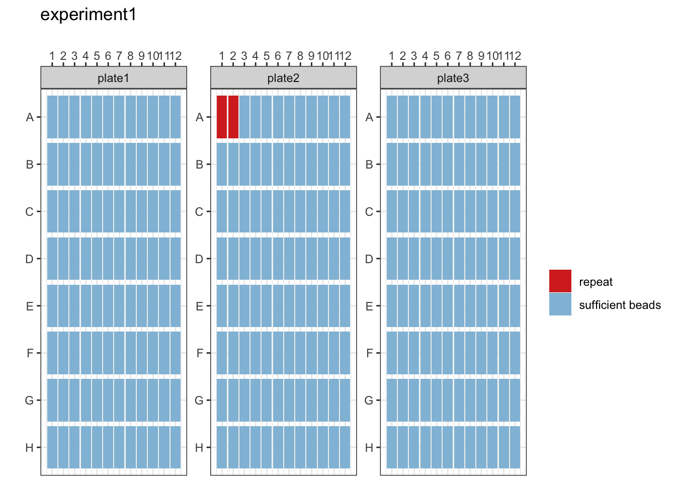
final_analysis[[4]] # Samples to repeat
#> # A tibble: 2 × 4
#>   Location SampleID Plate  QC
#>   <chr>    <chr>    <chr>  <chr>
#> 1 A1       Blank1   plate2 fail
#> 2 A2       Blank2   plate2 fail
1.2.1.4 Blanks QC Plot
final_analysis[[5]]![]()
1.2.1.5 Model Output Plot
final_analysis[[6]]
#> $plate1
#> Ignoring unknown labels:
#> • fill : "Antigen"
#>
#> $plate2
#> Ignoring unknown labels:
#> • fill : "Antigen"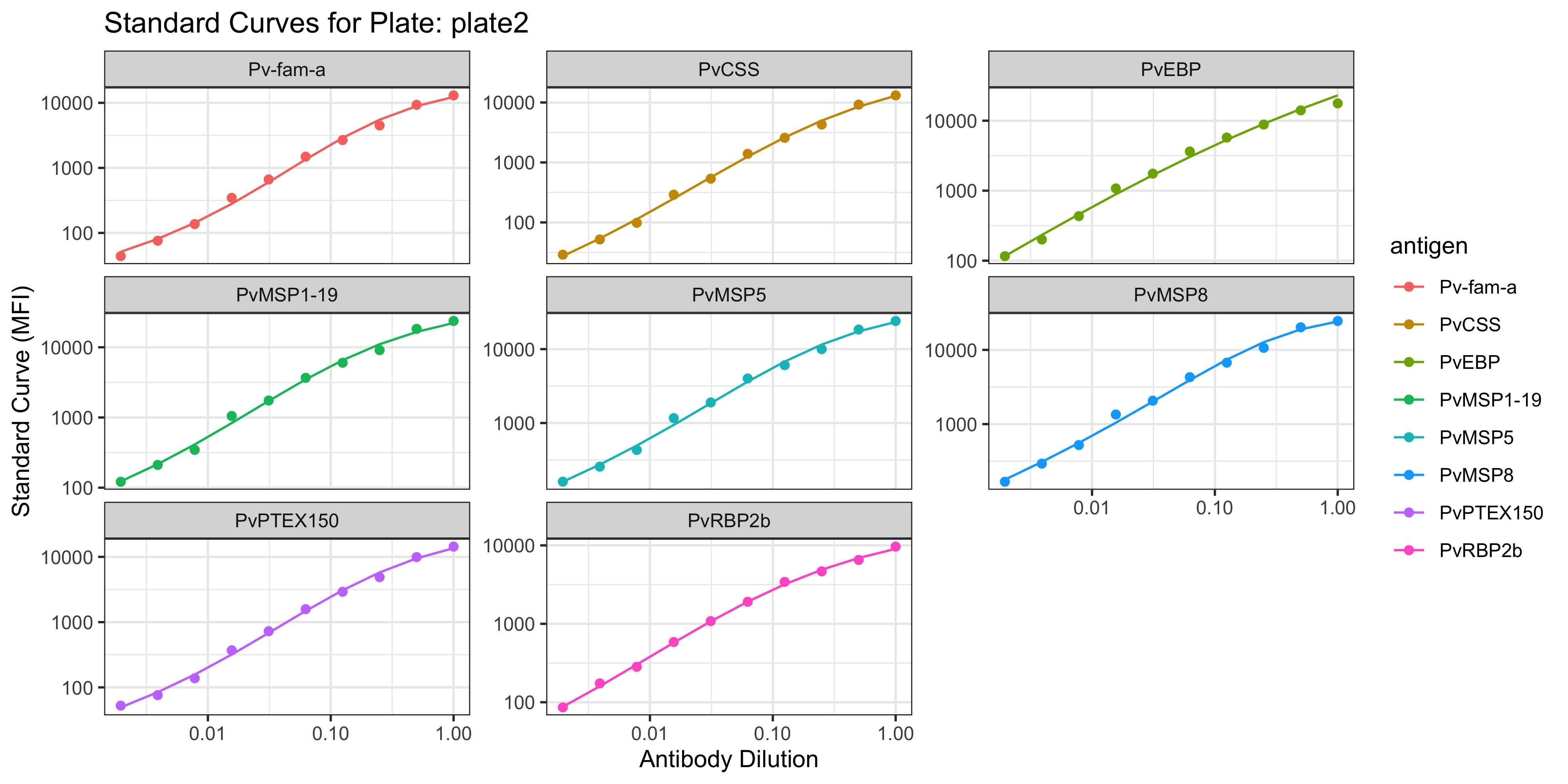
#>
#> $plate3
#> Ignoring unknown labels:
#> • fill : "Antigen"
1.2.2 Run Classification: No
no_classification_final_analysis <- runPvSeroPipeline(
  raw_data = your_raw_data,
  plate_layout = your_plate_layout,
  platform = "magpix",
  location = "ETH",
  experiment_name = "experiment1",
  std_point = 10,
  classify = "No", # key if you do NOT want any classification performed i.e., you do not have PvSeroTAT antigens
  algorithm_type = "antibody_model",
  sens_spec = "balanced"
)
#> PASS: File example_magpix_plate1.csv successfully validated.
#> PASS: File example_magpix_plate2.csv successfully validated.
#> PASS: File example_magpix_plate3.csv successfully validated.
#> Plate layouts correctly identified!
#> QC Processes completed.
#> MFI to RAU conversion completed.
#> Please write a standard point curve.
#> QC Plotting completed.
#> No Classification Performed.
1.2.2.1 MFI and RAU Data
no_classification_final_analysis[[1]]  %>%
  head() %>%
kable()| SampleID | Plate | QC_total | PvEBP_MFI | PvEBP_Dilution | Pv-fam-a_MFI | Pv-fam-a_Dilution | PvMSP5_MFI | PvMSP5_Dilution | PvMSP1-19_MFI | PvMSP1-19_Dilution | PvMSP8_MFI | PvMSP8_Dilution | PvPTEX150_MFI | PvPTEX150_Dilution | PvCSS_MFI | PvCSS_Dilution | PvRBP2b_MFI | PvRBP2b_Dilution |
|---|---|---|---|---|---|---|---|---|---|---|---|---|---|---|---|---|---|---|
| ABC013 | plate1 | pass | 2712 | 0.0003339 | 1569.0 | 0.0015045 | 673 | 0.0002163 | 327 | 0.0014567 | 182.0 | 1.95e-05 | 936.0 | 0.0001591 | 223 | 0.0000772 | 1068.0 | 0.0003714 |
| ABC014 | plate1 | pass | 134 | 0.0000216 | 378.0 | 0.0004204 | 117 | 0.0000277 | 197 | 0.0010331 | 58.0 | 1.95e-05 | 122.0 | 0.0000225 | 93 | 0.0000298 | 465.5 | 0.0001536 |
| ABC015 | plate1 | pass | 182 | 0.0000232 | 209.0 | 0.0002466 | 208 | 0.0000616 | 374 | 0.0015985 | 221.5 | 1.95e-05 | 293.0 | 0.0000535 | 868 | 0.0002235 | 463.0 | 0.0001527 |
| ABC016 | plate1 | pass | 152 | 0.0000222 | 229.5 | 0.0002688 | 101 | 0.0000244 | 89 | 0.0005994 | 48.0 | 1.95e-05 | 109.0 | 0.0000220 | 110 | 0.0000383 | 591.0 | 0.0001989 |
| ABC017 | plate1 | pass | 1135 | 0.0001478 | 236.0 | 0.0002758 | 299 | 0.0000950 | 507 | 0.0019840 | 209.5 | 1.95e-05 | 1665.5 | 0.0002668 | 266 | 0.0000893 | 671.0 | 0.0002277 |
| ABC018 | plate1 | pass | 174 | 0.0000229 | 395.0 | 0.0004370 | 175 | 0.0000460 | 78 | 0.0005452 | 70.0 | 1.95e-05 | 294.5 | 0.0000537 | 92 | 0.0000296 | 103.0 | 0.0000238 |
1.2.2.2 QC Plots
Repeat the same steps as above to find the QC plots!
#### Standard Curve Plot
no_classification_final_analysis[[2]]
#> NULL

#### Bead Counts QC Plot
no_classification_final_analysis[[3]] # Plot
no_classification_final_analysis[[4]] # Samples to repeat
#> # A tibble: 2 × 4
#>   Location SampleID Plate  QC
#>   <chr>    <chr>    <chr>  <chr>
#> 1 A1       Blank1   plate2 fail
#> 2 A2       Blank2   plate2 fail

#### Blanks QC Plot
no_classification_final_analysis[[5]]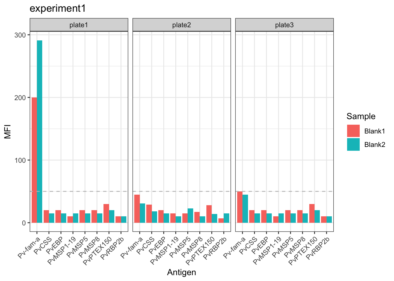
#### Model Output Plot
no_classification_final_analysis[[6]]
#> $plate1
#> Ignoring unknown labels:
#> • fill : "Antigen"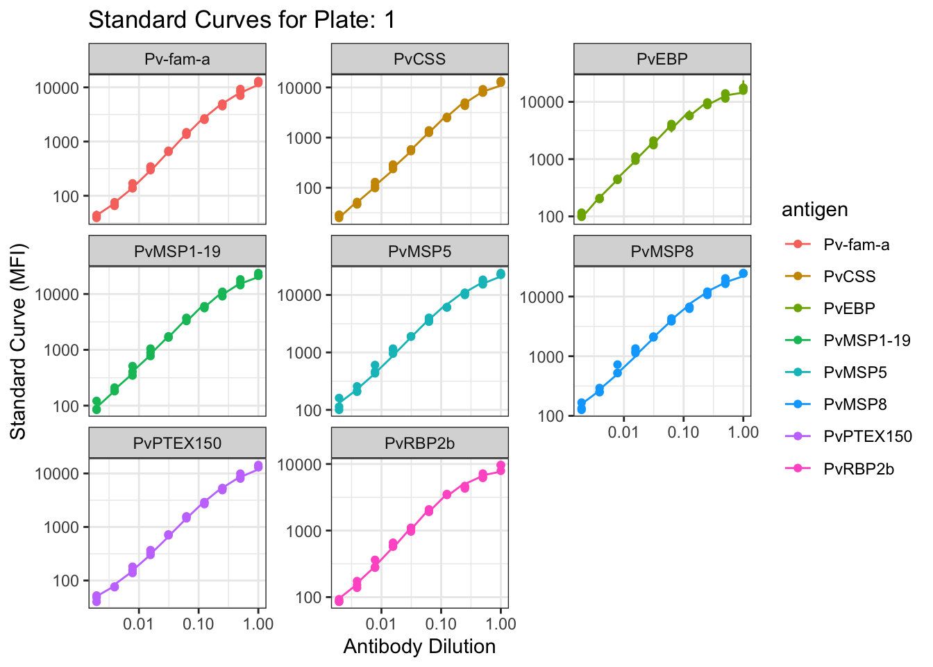
#>
#> $plate2
#> Ignoring unknown labels:
#> • fill : "Antigen"
#>
#> $plate3
#> Ignoring unknown labels:
#> • fill : "Antigen"
1.2.3 Create a PDF Report
renderQCReport(
  your_raw_data,
  your_plate_layout,
  "magpix",
  location = "ETH",
  path = "results/" # defaults to your current working directory
)